Brockschmidt, M. and Emmes, F. and Falke, S. and Fuhs, Carsten and Giesl,
J. (2016) Analyzing runtime and size complexity of integer programs. ACM
Transactions on Programming Languages and Systems 38 (4), pp. 1-50.
ISSN 0164-0925.
Downloaded from:
Usage Guidelines:
Please refer to usage guidelines at
or alternatively
Analyzing Runtime and Size Complexity of Integer Programs
Marc Brockschmidt, Microsoft Research Fabian Emmes, RWTH Aachen University Stephan Falke, Karlsruhe Institute of Technology Carsten Fuhs, Birkbeck, University of London J¨urgen Giesl, RWTH Aachen University
We present a modular approach to automatic complexity analysis of integer programs. Based on a novel alternation between finding symbolic time bounds for program parts and using these to infer bounds on the absolute values of program variables, we can restrict each analysis step to a small part of the program while maintaining a high level of precision. The bounds computed by our method are polynomial or exponential expressions that depend on the absolute values of input parameters.
We show how to extend our approach to arbitrary cost measures, allowing to use our technique to find upper bounds for other expended resources, such as network requests or memory consumption. Our contributions are implemented in the open source toolKoAT, and extensive experiments show the performance and power of our implementation in comparison with other tools.
Categories and Subject Descriptors: D.2.4 [Software Engineering]: Software/Program Verification; D.2.4 [Software Engineering]: Metrics; F.2.1 [Theory of Computation]: Analysis of Algorithms and Problem Complexity; F.3.1 [Theory of Computation]: Logics and Meanings of Programs
General Terms: Theory, Verification
Additional Key Words and Phrases: Runtime Complexity, Automated Complexity Analysis, Integer Programs
ACM Reference Format:
ACM Trans. Program. Lang. Syst. V, N, Article A (January YYYY), 48 pages. DOI = 10.1145/0000000.0000000 http://doi.acm.org/10.1145/0000000.0000000
1. INTRODUCTION
There exist numerous methods to prove termination of imperative programs, e.g., [Podelski and Rybalchenko 2004; Bradley et al. 2005; Cook et al. 2006; Albert et al. 2008; Alias et al. 2010; Harris et al. 2010; Spoto et al. 2010; Falke et al. 2011; Tsitovich et al. 2011; Bagnara et al. 2012; Brockschmidt et al. 2012; Ben-Amram and Genaim 2013; Brockschmidt et al. 2013; Cook et al. 2013; Larraz et al. 2013; Heizmann et al. 2014]. In many cases, however, termination is not sufficient, but the program should also terminate in reasonable (e.g.,
(pseudo-)polynomial) time. To prove bounds on a program’sruntime complexity, it is often
crucial to also derive (possibly non-linear) bounds on the size of program variables, which may be modified repeatedly in loops.
Supported by the DFG grant GI 274/6-1, the Air Force Research Laboratory (AFRL), the “Concept for the Future” of Karlsruhe Institute of Technology within the framework of the German Excellence Initiative, and the EPSRC.
Authors’ addresses: M. Brockschmidt: Microsoft Research, Cambridge, UK, F. Emmes: LuFG Informatik 2, RWTH Aachen University, Germany, S. Falke: (Current address) aicas GmbH, Karlsruhe, Germany, C. Fuhs: Dept. of Computer Science and Information Systems, Birkbeck, University of London, UK, J. Giesl: LuFG Informatik 2, RWTH Aachen University, Germany
Permission to make digital or hard copies of part or all of this work for personal or classroom use is granted without fee provided that copies are not made or distributed for profit or commercial advantage and that copies show this notice on the first page or initial screen of a display along with the full citation. Copyrights for components of this work owned by others than ACM must be honored. Abstracting with credit is permitted. To copy otherwise, to republish, to post on servers, to redistribute to lists, or to use any component of this work in other works requires prior specific permission and/or a fee. Permissions may be requested from Publications Dept., ACM, Inc., 2 Penn Plaza, Suite 701, New York, NY 10121-0701 USA, fax +1 (212) 869-0481, or [email protected].
c
YYYY ACM 0164-0925/YYYY/01-ARTA $10.00
whilei>0 do i:=i−1
done
whilex>0 do x:=x−1
done
whilei>0do i:=i−1
x:=x+i done
whilex>0do x:=x−1
done
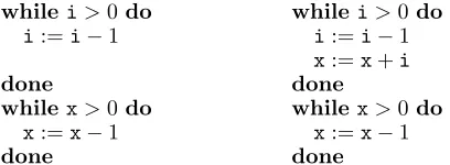
Fig. 1. Two similar programs with different runtime
Our approach to find such bounds builds upon the well-known observation that polynomial ranking functions for termination proofs also provide a runtime complexity bound [Alias et al. 2010; Albert et al. 2011a; Albert et al. 2012; Avanzini and Moser 2013; Noschinski
et al. 2013]. However, this only holds for proofs using asingle polynomial ranking function.
Larger programs are usually handled by a disjunctive [Lee et al. 2001; Cook et al. 2006; Tsitovich et al. 2011; Heizmann et al. 2014] or lexicographic [Bradley et al. 2005; Giesl et al. 2006; Fuhs et al. 2009; Alias et al. 2010; Harris et al. 2010; Falke et al. 2011; Brockschmidt et al. 2013; Cook et al. 2013; Larraz et al. 2013] combination of polynomial functions (we also refer to these components as “polynomial ranking functions”). Deriving a complexity bound in such cases is much harder.
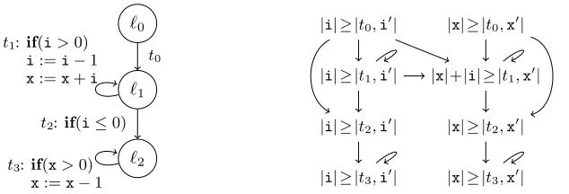
Example 1.1. Both programs in Fig. 1 can be proven terminating using the lexicographic
ranking function hi,xi. However, the program without the instruction “x :=x+i” has
linear runtime, while the program on the right has quadratic runtime. The crucial difference
between the two programs is in thesize ofxafter the first loop.
To handle such effects, we introduce a novel modular approach which alternates between
finding runtime bounds and findingsize bounds. In contrast to standard invariants, our size
bounds express a relation to the size of the variables at the program start, where we measure
the size of integersm∈Zby their absolute values |m| ∈N. Our method derives runtime
bounds for isolated parts of the program and uses these to deduce (often non-linear) size bounds for program variables at certain locations. Further runtime bounds can then be inferred using size bounds for variables that were modified in preceding parts of the program. By splitting the analysis in this way, we only need to consider small program parts in each step, and the process is repeated until all loops and variables have been handled.
As an example, for the second program in Fig. 1, our method proves that the first loop is
executed linearly often using the ranking function i. Then, it deduces thatiis bounded by
the size |i0| of its initial valuei0in all iterations of this loop. Combining these bounds, it
infers thatxis incremented by a value bounded by|i0|at most|i0|times in the first loop,
i.e.,xis bounded by the sum of its initial size|x0|and|i0|2. Finally, our method detects that
the second loop is executed xtimes, and combines this with our bound|x0|+|i0|2 onx’s
value when entering the second loop. In this way, we can infer the bound|i0|+|x0|+|i0|2
for the program’s runtime.1 This novel combination of runtime and size bounds allows us
to handle loops whose runtime depends on variables like xthat were modified in earlier
loops (where the values of these variables can also be modified in a non-linear way). Thus, our approach succeeds on many programs that are beyond the reach of previous techniques based on the use of ranking functions.
Sect. 2 introduces the basic notions for our approach. Then Sect. 3 and Sect. 4 present our techniques to compute runtime and size bounds, respectively. In Sect. 5, we extend our approach to handle possibly recursive procedure calls. Finally, we show in Sect. 6 how
1Since each step of our method over-approximates the runtime or size of a variable, we actually obtain the
[image:3.612.207.411.93.168.2]Input:List x
`0:List y:=null
`1:while x6=null do y:=new List(x.val,y)
x:=x.next done
List z:=y
`2:while z6=null do List u:=z.next
`3: while u6=null do z.val :=z.val+u.val u:=u.next
done z:=z.next done
Input:int x
`0:int y:= 0
`1:while x>0 do y:=y+ 1
x:=x−1
done int z:=y
`2:while z>0 do int u:=z−1
`3: whileu>0 do skip
u:=u−1
done z:=z−1
done
`0
`1
`2
`3
t0:y:= 0
t1:if(x>0) y:=y+ 1
x:=x−1
t2:if(x≤0) z:=y
t3:if(z>0) u:=z−1
t4:if(u>0) if(z>0)
u:=u−1
t5:if(u≤0) if(z>0)
z:=z−1
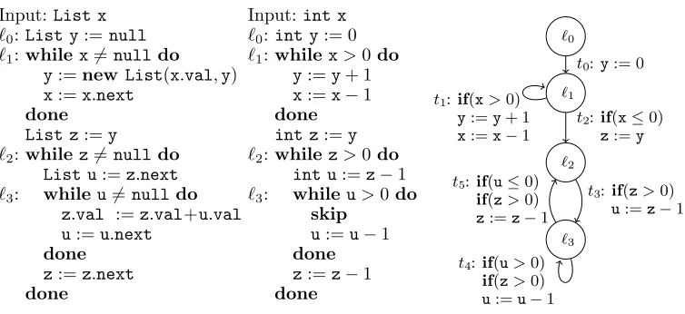
Fig. 2. List processing program, its integer abstraction, and a graph representation of the integer abstraction
a generalization to arbitrary cost measures can be used to obtain a modular analysis of procedures. Such cost measures can also express resource usage such as network requests. In Sect. 7, we compare our technique to related work and show its effectiveness in an extensive experimental evaluation. We conclude in Sect. 8, discussing limitations, possible further extensions, and applications of our method. All proofs are given in App. A.
A preliminary version of parts of this paper was published earlier [Brockschmidt et al. 2014]. It is extended substantially in the present paper:
— We present new techniques to automatically synthesize bounds for programs with an exponential growth of data sizes in Sect. 4.
— We extend our approach to programs with recursion in Sect. 5 and show how to also infer exponential runtime bounds for such programs.
— We generalize our technique to analyze complexity w.r.t. arbitrary cost measures in Sect. 6.1.
— We extend the modularity of our analysis such that program parts (e.g., library procedures) can be handled completely independently in Sect. 6.2.
— We integrated these new contributions in our prototype implementationKoATand present
an extensive evaluation, comparing it to recently developed competing tools in Sect. 7.3.
KoAT is now also available as free software, allowing to easily experiment with extensions
to our framework.
— We give detailed proofs for all theorems in App. A.
2. PRELIMINARIES
We regard sequential imperative integer programs with (potentially non-linear) arithmetic and unbounded non-determinism.
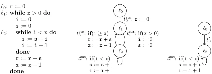
Example 2.1. In Fig. 2, a list processing program is shown on the left. For an input list
x, the loop at location`1creates a listyby reversing the elements ofx. The loop at location
`2 iterates over the listyand increases each element by the sum of its successors. So ify
was [5,1,3], it will be [5 + 1 + 3,1 + 3,3] after the second loop.
In the middle of Fig. 2, an integer abstraction of our list program is shown. Here, list variables are replaced by integers that correspond to the length of the replaced list. Such
integer abstractions can be obtained automatically using tools such asCOSTA[Albert et al.
[image:4.612.121.498.90.263.2]We fix a (finite) set of program variablesV ={v1, . . . , vn}and represent integer programs
as directed graphs. Nodes are program locations Land edges are program transitions T.
The setLcontains acanonical start location`0. W.l.o.g., we assume that no transition leads
back to`0. All transitions originating in`0 are calledinitial transitions. The transitions are
labeled by formulas over the variablesV and primed post-variablesV0 ={v10, . . . , vn0} which represent the values of the variables after the transition. In the graph on the right of Fig. 2,
we represented these formulas by sequences of instructions. For instance,t3 is labeled by
the formula z>0∧u0 =z−1∧x0=x∧y0 =y∧z0 =z. In our example, we used standard
invariant-generation techniques (based on the Octagon domain [Min´e 2006]) to propagate
simple integer invariants, adding the conditionz>0 to the transitionst4 andt5.
Definition2.2 (Programs). Atransition is a tuple (`, τ, `0) where`, `0∈ Lare locations
andτ is a quantifier-free formula relating the (pre-)variablesV and the post-variablesV0.
Aprogram is a set of transitionsT. A configuration (`,v) consists of a location`∈ L and avaluation v:V →Z. We write (`,v)→t(`0,v0) for anevaluation step with a transition
t= (`, τ, `0) iff the valuationsv,v0 satisfy the formulaτ oft. As usual, we say thatv,v0 satisfy a quantifier-free formulaτ over the variablesV ∪ V0 iffτ becomes true when every
v ∈ V is instantiated by the number v(v) and every v0 ∈ V0 is instantiated byv0(v). We
drop the indextin “→t” when that information is not important and write (`,v)→k (`0,v0) if (`0,v0) is reached from (`,v) ink evaluation steps.
For the program of Ex. 2.1, we have (`1,v1) →t2 (`2,v2) for any valuations v1 and
v2 where v1(x) = v2(x) ≤ 0, v1(y) = v2(y) = v2(z), and v1(u) = v2(u). Note that in
our representation, every location can potentially be a “final” one (if none of its outgoing transitions is applicable for the current valuation).
LetT always denote the analyzed program. Our goal is to find bounds on the runtime and
the sizes of program variables, where these bounds are expressed as functions in the sizes of the input variablesv1, . . . , vn. For our example, our approach will detect that its runtime is bounded by 3 + 4· |x|+|x|2(i.e., it is quadratic in|x|). We measure thesize of variable values
v(vi) by their absolute values|v(vi)|. For a valuationvand a vectorm= (m1, . . . , mn)∈Nn,
letv≤mabbreviate|v(v1)| ≤m1∧. . .∧ |v(vn)| ≤mn. We define theruntime complexity
of a program T by a function rc that maps sizesmof program variables to the maximal
number of evaluation steps that are possible from an initial configuration (`0,v) withv≤m.
Definition2.3 (Runtime Complexity). Theruntime complexity rc :Nn →N∪ {ω}of a
programT is defined as rc(m) = sup{k∈N| ∃v0, `,v.v0≤m∧(`0,v0)→k(`,v)}.
Here, rc(m) =ω means non-termination or arbitrarily long runtime. Programs with
arbi-trarily long runtime can result from non-deterministic value assignment, e.g.,i:=nondet();
whilei>0doi:=i−1 done.
To analyze complexity in a modular way, we construct a runtime approximation Rsuch
that for anyt∈ T,R(t) over-approximates the number of times that tcan be used in an
evaluation. As we generate new bounds by composing previously found bounds, we only use
weakly monotonic functionsR(t), i.e., wheremi ≥m0i implies (R(t))(m1, . . . , mi, . . . , mn)≥ (R(t))(m1, . . . , m0i, . . . , mn)). We define the set ofupper boundsUB as the weakly monotonic
functions from Nn →
Nand ω. Here, “ω” denotes the constant function which maps all
arguments m∈Nn toω. We have ω > n for alln∈N. In our implementation, we use a
subset UB0(UB that is particularly suitable for the automated synthesis of bounds. We
also allow an application of functions from UB0 to integers instead of naturals by taking
their absolute value. More precisely, UB0 is the smallest set for which the following holds:
— |v| ∈UB0 forv∈ V (variables)
— ω∈UB0 (unbounded function)
— P
1≤i≤k ai · Q1≤j≤mifi,j
— max{f1, . . . , fk} ∈ UB0, min{f1, . . . , fk} ∈ UB0 for f1, . . . , fk ∈ UB0 (maximum and minimum)
— kf∈UB0 fork
∈N,f ∈UB0 (exponentials)
Thus, UB0 is closed under addition, multiplication, maximum, minimum, and exponentiation
(using natural numbers as bases). These closure properties will be used when combining bound approximations in the remainder of the paper.
We now formally define our notion of runtime approximations. Here, we use →∗◦ →
t to denote the relation describing arbitrary many evaluation steps followed by a step with transitiont.
Definition2.4 (Runtime Approximation). A functionR:T →UB is aruntime approxi-mation iff (R(t))(m)≥sup{k∈N| ∃v0, `,v.v0≤m∧(`0,v0) (→∗◦ →t)k(`,v)}holds for
all transitions t∈ T and allm ∈Nn. We then say that R(t) is aruntime bound for the
transition t. Theinitial runtime approximation R0 is defined as R0(t) = 1 for all initial
transitionst andR0(t) =ωotherwise. Here, “1” denotes the constant function which maps
all argumentsm∈Nn to 1.
We can combine the approximations for individual transitions represented by R(t) to
obtain a bound for the runtime complexity rc of the whole programT. Here forf, g∈UB,
the comparison, addition, multiplication, maximum, and the minimum are defined
point-wise. So f ≥ g holds iff f(m) ≥ g(m) for all m ∈ Nn and f +g is the function with
(f+g)(m) =f(m) +g(m), whereω+n=ω for alln∈N∪ {ω}.
Remark2.5 (Approximatingrc). Let R be a runtime approximation for T. Then
P
t∈T R(t)≥rc.
The overall boundP
t∈T R(t) = 3 + 4· |x|+|x|2 for the program in Ex. 2.1 was obtained
in this way.
For size complexity, we analyze how large the value of a program variable can become.
Analogous toR, we use asize approximation S, whereS(t, v0) is a bound on the size of the
variablev after a certain transitiont was used in an evaluation. For any transitiont∈ T
andv∈ V, we call|t, v0| aresult variable. Later, we will build aresult variable graph (RVG),
whose nodes are result variables and whose edges represent the flow of data in our program.
Definition2.6 (Result Variables and Size Approximation). LetRV={|t, v0| |t∈ T, v∈
V} be the set of result variables. A function S : RV → UB is a size approximation iff
(S(t, v0))(m) ≥ sup{|v(v)| | ∃v
0, `,v.v0 ≤ m∧(`0,v0) (→∗◦ →t) (`,v)} holds for all
|t, v0| ∈RVand allm∈Nn. We then say that S(t, v0) is asize bound for the result variable |t, v0|. The initial size approximation S0 is defined asS0(t, v0) =ω for all |t, v0| ∈RV. A
pair (R,S) is acomplexity approximation ifRis a runtime approximation andS is a size
approximation.
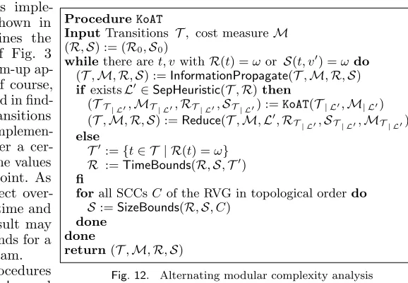
Our method performs an iterative refinement of runtime and size approximations. The
general overall procedure is displayed in Fig. 3.2 It starts with the initial approximations
(R,S) := (R0,S0)
whilethere aret, vwithR(t) =ωorS(t, v0) =ωdo T0:={t∈ T | R(t) =ω}
R :=TimeBounds(R,S,T0)
forall SCCsCof the RVG in topological orderdo S:=SizeBounds(R,S, C)
done done
Fig. 3. Alternating complexity analysis procedure
R0,S0 and then loops until time bounds
for all transitions and size bounds for all result variables have been found. In each iteration, it first calls the sub-procedure
TimeBounds (cf. Sect. 3) to improve the
runtime bounds for those transitions T0
for which we have no bound yet. Then, the
procedureSizeBounds(cf. Sect. 4) is used
to obtain new size bounds, using the time bounds computed so far. It processes strongly connected components (SCCs) of the result variable graph, corresponding to sets of variables
which influence each other.3In the next iteration of the main outer loop, TimeBoundscan
then use the newly obtained size bounds. In this way, the procedures for inferring runtime and size complexity alternate, allowing them to make use of each other’s results. The procedure is aborted when in one iteration of the outer loop no new bounds could be found.
3. COMPUTING RUNTIME BOUNDS
To find runtime bounds automatically, we usepolynomial ranking functions (PRFs). Such
ranking functions are widely used in termination analysis and many techniques are available to generate PRFs automatically [Podelski and Rybalchenko 2004; Bradley et al. 2005; Fuhs et al. 2007; Fuhs et al. 2009; Alias et al. 2010; Falke et al. 2011; Bagnara et al. 2012; Ben-Amram and Genaim 2013; Leike and Heizmann 2014]. While most of these techniques only generate linear PRFs, the theorems of this section hold for general polynomial ranking functions as well. In our analysis framework, we repeatedly search for PRFs for different parts of the program, and the resulting combined complexity proof is analogous to the use of lexicographic combinations of ranking functions in termination analysis.
In Sect. 3.1 we recapitulate the basic approach to use PRFs for the generation of time bounds. In Sect. 3.2, we improve it to a novel modular approach which infers time bounds by combining PRFs with information about variable sizes and runtime bounds found earlier.
3.1. Runtime Bounds from Polynomial Ranking Functions
A PRF Pol : L → Z[v1, . . . , vn] assigns an integer polynomial Pol(`) over the program
variables to each location `. Then configurations (`,v) are measured as the value of the
polynomialPol(`) for the numbersv(v1), . . . ,v(vn). To obtain time bounds, we search for
PRFs where no transition increases the measure of configurations, and at least one transition decreases it. To rule out that this decrease continues forever, we also require that the measure
has a lower bound. As mentioned before Def. 2.2, here the formula τ of a transition (`, τ, `0)
may have been extended by suitable program invariants.
Definition3.1 (PRF). We call Pol : L → Z[v1, . . . , vn] a polynomial ranking function
(PRF) forT iff there is a non-emptyT⊆ T such that the following holds:
• for all (`, τ, `0)∈ T, we have τ⇒(Pol(`))(v1, . . . , vn)≥(Pol(`0))(v10, . . . , vn0)
• for all (`, τ, `0)∈ T, we haveτ⇒(Pol(`))(v1, . . . , vn)>(Pol(`0))(v01, . . . , vn0) andτ⇒(Pol(`))(v1, . . . , vn)≥1
The constraints on a PRF Pol are the same as the constraints of Bradley et al. [2005]
needed for finding ranking functions for termination proofs. Hence, this allows to re-use
existing PRF synthesis techniques and tools. They imply that the transitions inT can only
be used a limited number of times, as each application of a transition fromT decreases
the measure, and no transition increases it. Hence, if the program is called with input
m1, . . . , mn, no transitiont∈ T can be used more often than (Pol(`0))(m1, . . . , mn) times.
Consequently,Pol(`0) is a runtime bound for the transitions inT. Note that no such bound
is obtained for the remaining transitions in T.
Example 3.2. To find bounds for the program in Ex. 2.1, we usePol1 withPol1(`) =x
for all ` ∈ L, i.e., we measure configurations by the value of x. No transition increases
this measure and t1 decreases it. The conditionx>0 ensures that the measure is positive
whenevert1 is used, i.e., T={t1}. HencePol1(`0) (i.e., the valuexat the beginning of
the program) is a bound on the number of timest1can be used.
3The result variable graph will be introduced in Sect. 4. As we will discuss in Sect. 4, proceeding in topological
Such PRFs lead to a basic technique for inferring time bounds. As mentioned in Sect. 2, to obtain a modular approach, we only allow weakly monotonic functions as complexity bounds. For any polynomialp∈Z[v1, . . . , vn], let [p] result frompby replacing all coefficients and variables with their absolute value (e.g., forPol1(`0) =xwe have [Pol1(`0)] =|x|and
if p = 2·v1−3·v2 then [p] = 2· |v1|+ 3· |v2|). As [p](m1, . . . , mn) ≥ p(m1, . . . , mn) holds for all m1, . . . , mn∈Z, this is a sound approximation, and [p] is weakly monotonic.
In our example, the initial runtime approximation R0 can now be refined to R1, with
R1(t1) = [Pol1(`0)] =|x|andR1(t) =R0(t) for all other transitionst. Thus, this provides a
first basic method for the improvement of runtime approximations.
Theorem3.3 (Complexities from PRFs). LetRbe a runtime approximation and Pol be a PRF for T. Let R0(t) = [Pol(`
0)] for all t∈ T and R0(t) =R(t) for all other
t∈ T. Then,R0 is also a runtime approximation.
To ensure that R0(t) is at most as large as the previous bound R(t) in Thm. 3.3, one
could also define R0(t) = min{[Pol(`
0)],R(t)}. A similar improvement is possible for all
other techniques in the paper that refine the approximationsRorS.
3.2. Modular Runtime Bounds from PRFs and Size Bounds
Using Thm. 3.3 repeatedly to infer complexity bounds for all transitions in a program only succeeds for simple algorithms. In particular, it often fails for programs with non-linear runtime. Although corresponding SAT- and SMT-encodings exist [Fuhs et al. 2007],
generating a suitable PRFPol of a non-linear degree is a complex synthesis problem (and
undecidable in general). This is aggravated by the need to consider all ofT at once, which
is required to check that no transition ofT increasesPol’s measure.
Therefore, we now present a newmodular technique that only considers isolated program
parts T0⊆ T in each PRF synthesis step. The bounds obtained from these “local” PRFs are then lifted to a bound expressed in the input values. To this end, we combine them with
bounds on the size of the variables when entering the program part T0 and with a bound
on the number of times thatT0 can be reached in evaluations of the full programT. This
allows us to use existing efficient procedures for the automated generation of (often linear) PRFs for the analysis of programs with possibly non-linear runtime.
Example 3.4. We continue Ex. 3.2 and consider the subset T01 = {t1, . . . , t5} ⊆ T.
Using the constant PRFPol2 withPol2(`1) = 1 andPol2(`2) =Pol2(`3) = 0, we see that
t1, t3, t4, t5do not increase the measure of configurations and that t2 decreases it. Hence, in
executions that are restricted to T01 and that start in`1, t2 is used at most [Pol2(`1)] = 1
times. To obtain a global result, we consider how oftenT01 is reached in a full program run.
AsT01is only reached by the transitiont0, wemultiply its runtime approximationR1(t0) = 1
with the local bound [Pol2(`1)] = 1 obtained for the sub-program T01. Thus, we refineR1 to R2(t2) =R1(t0)·[Pol2(`1)] = 1·1 = 1 and we setR2(t) =R1(t) for all othert.4
In general, to estimate how often a sub-programT0 is reached in an evaluation, we consider
the transitions ˜t∈ T \ T0 that lead to the “entry location”` of a transition fromT0. We
multiply the runtime bound of such transitions ˜t (expressed in terms of the input variables)
with the bound [Pol(`)] for runs starting in`. This combination is an over-approximation
4The choice ofT0
1={t1, . . . , t5}does not quite match our procedure in Fig. 3, where we would only generate a PRF for those transitionsT0={t∈ T | R
1(t) =ω}for which we have no bound yet. So instead ofT01 we would useT00
1 ={t2, . . . , t5}. However, this would result in a worse upper bound, becauseT001 is reached by both transitionst0andt1. Thus, we would obtainR2(t2) =R1(t0)·[Pol2(`1)]+R1(t1)·[Pol2(`1)] = 1+|x|. To obtain better bounds, our implementation uses an improved heuristic to chooseT0in the procedure of Fig. 3: After generating a PRFPolfor the transitionsT0without bounds,T0is extended by all further transitions (`, τ, `0)∈ T \ T0wherePolis weakly decreasing, i.e., whereτ⇒(Pol(`))(v
1, . . . , vn)≥(Pol(`0))(v10, . . . , v0n)
holds. Thus, our implementation would extendT00 1 toT
0 1=T
of the overall runtime, as the runtime of individual runs may differ greatly. We present an improved treatment of this problem in Sect. 6.2. More generally, capturing such effects is
treated in amortized complexity analysis (see, e.g., [Hoffmann et al. 2012; Sinn et al. 2014]).
In our example, t0 is the only transition leading toT01={t1, . . . , t5}and thus, the runtime
boundR1(t0) = 1 is multiplied with [Pol2(`1)].
Example 3.5. We continue Ex. 3.4 and consider the transitions T02 = {t3, t4, t5} for
which we have found no bound yet. Then Pol3(`2) =Pol3(`3) =zis a PRF forT02 with
(T02)={t5}. Sorestricted to the sub-program T02, t5 is used at most [Pol3(`2)] =|z|times.
Here, zrefers to the value when enteringT02 (i.e., after transitiont2).
To translate this bound into an expression in the input values of the whole programT,
we substitute the variablezby its maximal size after using the transition t2, i.e., by the
size bound S(t2,z0). As the runtime of the loop at`2depends on the size ofz, our approach
alternates between computing runtime and size bounds. Our method to compute size bounds will determine that the size ofzafter the transitiont2 is at most|x|, cf. Sect. 4. Hence, we
replace the variablezin [Pol3(`2)] =|z|byS(t2,z0) =|x|. To compute a global bound, we
also have to examine how oftenT02 can be executed in a full program run. AsT
0
2 is only
reached byt2, we obtainR3(t5) =R2(t2)· |x|= 1· |x|=|x|. For all other transitionst, we
again have R3(t) =R2(t).
In general, the polynomials [Pol(`)] for the entry locations`ofT0 only provide a bound
in terms of the variable values at location`. To find bounds expressed in the variable values
at the start location`0, we use oursize approximation S and replace all variables in [Pol(`)]
by our approximation for their sizes at location `. For this, we define the application of
polynomials to functions. Letp∈N[v1, . . . , vn] andf1, . . . , fn ∈UB. Thenp(f1, . . . , fn) is the
function with (p(f1, . . . , fn))(m) =p(f1(m), . . . , fn(m)) for allm∈Nn. Weak monotonicity
ofp, f1, . . . , fn also implies weak monotonicity ofp(f1, . . . , fn), i.e.,p(f1, . . . , fn)∈UB.
In Ex. 3.5, we applied the polynomial [Pol3(`2)] for the location`2ofT02to the size bounds S(t2, v0) for the variablesx,y,z,u(i.e., to their sizes before enteringT02). As [Pol3(`2)] =|z|
andS(t2,z0) =|x|, we obtained [Pol3(`2)](S(t2,x0),S(t2,y0),S(t2,z0),S(t2,u0)) =|x|.
Our technique is formalized as the procedure TimeBounds in Thm. 3.6. It takes the
current complexity approximation (R,S) and a sub-program T0, and computes a PRF for
T0. Based on this, R is refined to the approximation R0. In the following theorem, for
any location `, letT` contain all transitions (˜`,˜τ , `)∈ T \ T0 leading to `. Moreover, let
L0={`| T`6=∅∧ ∃`0.(`, τ, `0)∈ T0} contain all entry locations ofT0.
Theorem 3.6 (TimeBounds). Let (R,S) be a complexity approximation, let T0 ⊆ T such that T0 contains no initial transitions, and let Pol be a PRF for T0. Let R0(t) = P
`∈L,0˜t∈T`R(˜t)·[Pol(`)](S(˜t, v
0
1), . . . ,S(˜t, vn0)) for t ∈ T
0
and R0(t) = R(t) for all t ∈ T \ T0. Then,TimeBounds(R,S,T0) =R0 is also a runtime approximation.
Here one can see why we require complexity bounds to be weakly monotonic. The reason
is that S(˜t, v0) over-approximates the size ofv at some location `. Hence, to ensure that
[Pol(`)](S(˜t, v0
1), . . . ,S(˜t, v0n)) correctly over-approximates how often transitions ofT
0 can
be applied in parts of evaluations that only use transitions fromT0, [Pol(`)] must be weakly monotonic.
Example 3.7. We use Thm. 3.6 to obtain bounds for the transitions not handled in Ex. 3.5. For T03={t3, t4}, we usePol4(`2) = 1,Pol4(`3) = 0, and hence (T30)={t3}. The
transitionst2andt5lead toT03, and thus, we obtainR4(t3) =R3(t2)·1 +R3(t5)·1 = 1 +|x|
andR4(t) =R3(t) for all other transitionst.
ForT04={t4}, we usePol5(`3) =uwith (T04)=T04. The partT04is only entered by the
we will determineS(t3,u0) =|x|). Thus,R5(t4) =R4(t3)· S(t3,u0) = (1 +|x|)· |x|=|x|+|x|2
andR5(t) =R4(t) for all othert∈ T. So while the runtime ofT04on its own is linear, the loop
at location`3is reached a linear number of times, i.e., its transition t4 is usedquadratically
often. Thus, the overall program runtime is bounded byP
t∈TR5(t) = 3 + 4· |x|+|x|2. 4. COMPUTING SIZE BOUNDS
The procedureTimeBoundsimproves the runtime approximationR, but up to now the size
approximationS was only used as an input. To infer bounds on the size of variables, we
proceed in three steps. First, we findlocal size boundsthat approximate the effect of a single
transition on the sizes of variables. Then, we construct aresult variable graph that makes
the flow of data between variables explicit. Finally, we analyze each strongly connected component (SCC) of this graph independently. Here, we combine our runtime approximation
Rwith the local size bounds to estimate how often transitions modify a variable value.
To describe how the size of a post-variablev0 is related to the pre-variables of a transition
t, we use local size boundsSl(t, v0).5 Thus,S(t, v0) is a bound on the size ofv after usingt
expressed in the sizes of the program inputs, and Sl(t, v0) is a bound expressed in the sizes
of the pre-variables of t. In most cases, such local size bounds can be inferred directly from
the formula of the transition (e.g., if it contains sub-formulas such as x0 =x+ 1). For the
remaining cases, we use SMT solving to find bounds from certain classes of templates (cf. Sect. 4.2).
Definition4.1 (Local Size Approximation). We call Sl : RV →UB a local size
approx-imation iff (Sl(t, v0))(m) ≥ sup{|v0(v)| | ∃`,v, `0,v0.v ≤ m∧(`,v) →t (`0,v0)} for all
|t, v0| ∈RVand allm∈Nn.
Example 4.2. For the program of Ex. 2.1, we have Sl(t1,y0) =|y|+ 1, as t1 increases yby 1. Similarly, |t1,x0|is bounded by |x|ast1 is only executed ifxis positive and thus
decreasing xby 1 does not increase itsabsolute value.
To track how variables influence each other, we construct a result variable graph (RVG) whose nodes are the result variables. The RVG has an edge from a result variable|t,˜v˜0| to |t, v0| if the transition ˜t can be used immediately beforetand if ˜v occurs in the local size boundSl(t, v0). Such an edge means that the size of ˜v0 in the post-location of the transition ˜
t may influence the size ofv0 in t’s post-location.
To state which variables may influence a function f ∈UB, we define itsactive variables
as actV(f) = {vi ∈ V | ∃m1, . . . , mn, m0i ∈N.f(m1, . . . , mi, . . . , mn) =6 f(m1, . . . , m0i, . . . ,
mn)}. To computeactV(f) for the upper boundsf ∈UB0 in our implementation, we simply
take all variables occurring inf.
Letpre(t) denote the transitions that may precedetin evaluations, i.e.,pre(t) ={˜t∈ T |
∃v0, `,v.(`0,v0)→∗◦ →˜t◦ →t(`,v)}. While pre(t) is undecidable in general, there exist several techniques to compute over-approximations, cf. [Fuhs et al. 2009; Falke et al. 2011].
Definition4.3 (RVG). Let Sl be a local size approximation. AnRVG has T’s result variables as nodes and the edges{(|˜t,v˜0|,|t, v0|)|t˜∈pre(t),v˜∈actV(Sl(t, v0))}.
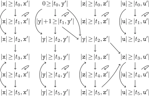
Example 4.4. The RVG for the program from Ex. 2.1 is shown in Fig. 4. Here, we display
local size bounds in the RVG to the left of the result variables, separated by “≥” (e.g.,
“|x| ≥ |t1,x0|” meansSl(t1,x0) =|x|). As we haveSl(t2,z0) =|y|for the transitiont2, which
setsz:=y, we concludeactV(Sl(t2,z0)) ={y}. The program graph impliespre(t2) ={t0, t1},
and thus, the RVG contains edges from|t0,y0|to|t2,z0|and from|t1,y0| to|t2,z0|.
5So the subscript “l” inS
|x| ≥ |t0,x0| 0≥ |t0,y0| |z| ≥ |t0,z0| |u| ≥ |t0,u0|
|x| ≥ |t1,x0| |y|+1≥ |t1,y0| |z| ≥ |t1,z0| |u| ≥ |t1,u0|
|x| ≥ |t2,x0| |y| ≥ |t2,y0| |y| ≥ |t2,z0| |u| ≥ |t2,u0|
|x| ≥ |t3,x0| |y| ≥ |t3,y0| |z| ≥ |t3,z0| |z| ≥ |t3,u0|
|x| ≥ |t4,x0| |y| ≥ |t4,y0| |z| ≥ |t4,z0| |u| ≥ |t4,u0|
|x| ≥ |t5,x0| |y| ≥ |t5,y0| |z| ≥ |t5,z0| |u| ≥ |t5,u0|
Fig. 4. Result variable graph for the program from Ex. 2.1
SCCs of the RVG represent sets of result variables that may influence each other. To lift
the local approximationSl to a global one, we consider each SCC on its own. We treat the
SCCs in topological order, reflecting the data flow. In this way when computing size bounds for an SCC, we already have the size bounds available for those result variables that the current SCC depends on. As usual, an SCC is a maximal subgraph with a path from each
node to every other node. An SCC istrivial if it consists of a single node without an edge
to itself. In Sect. 4.1, we show how to deduce global bounds for trivial SCCs and in Sect. 4.2, we handle non-trivial SCCs where transitions are applied repeatedly.
4.1. Size Bounds for Trivial SCCs of the RVG
Sl(t, v0) approximates the size of v0 after the transitiont w.r.t.t’s pre-variables, but our goal is to obtain aglobal boundS(t, v0) that approximatesv0 w.r.t. the initial values of the
variables at the program start. For trivial SCCs that consist of a result variableα=|t, v0|
with an initial transitiont, the local boundSl(α) is also the global boundS(α), as the start
location`0 has no incoming transitions.
Next, we consider trivial SCCs α=|t, v0|with incoming edges from other SCCs. Here,
Sl(α) (m) is an upper bound on the size ofv0 after using the transitiontin a configuration
where the sizes of the variables are at mostm. To obtain a global bound, we replace mby
upper bounds ont’s input variables. The edges leading toαcome from result variables|˜t, v0
i| where ˜t∈pre(t) and thus, a bound for the result variableα=|t, v0|is the maximum of all applications of Sl(α) toS(˜t, v10), . . . ,S(˜t, vn0), for all ˜t∈pre(t).
Example 4.5. Consider the RVG of Ex. 4.4 in Fig. 4, for which we want to find size bounds. For the trivial SCC {|t0,y0|}, we have 0 ≥ |t0,y0|, and thus we set S(t0,y0) = 0.
Similarly, we obtainS(t0,x0) =|x|. Finally, consider the local size bound|y| ≥ |t2,z0|. To
express this bound in terms of the input variables, we consider the predecessors |t0,y0|
and |t1,y0| of |t2,z0|. So Sl(t2,z0) must be applied to S(t0,y0) and S(t1,y0). If SCCs are
handled in topological order, one already knows thatS(t0,y0) = 0 andS(t1,y0) =|x|. Hence, S(t2,z0) = max{0,|x|}=|x|.
Thm. 4.6 presents the resulting procedureSizeBounds. Based on the current approximation
(R,S), it improves the global size bound for the result variable in a trivial SCC of the RVG.
Theorem4.6 (SizeBounds for Trivial SCCs). Let (R,S) be a complexity
approxi-mation, letSl be a local size approximation, and let{α} ⊆RVbe a trivial SCC of the RVG.
We define S0(α0) =S(α0)forα0 6=αand
• S0(α) =Sl(α), ifα=|t, v0|for some initial transition t
• S0(α) = max{ Sl(α) (S(˜t, v01), . . . ,S(˜t, v0n)) |˜t∈pre(t)}, otherwise.
ThenSizeBounds(R,S,{α}) =S0 is also a size approximation.
4.2. Size Bounds for Non-Trivial SCCs of the RVG
Finally, we show how to improve the size bounds for result variables in non-trivial SCCs of
the RVG. Such an SCCC corresponds to the information flow in a loop and hence, each of
its local changes can be applied several times. To approximate the overall effect of these
repeated changes for a transitiont ofC, we combine the time boundR(t) with the local
size boundsSl(t, v0). Then, to approximate the effect of the whole SCCC, we combine the
bounds obtained for all transitionstofC. To simplify this approximation, we classify result
variablesαinto three sets=,. u, and ˙×, depending on their local size boundSl(α):
• α ∈ = (. α is an “equality”) if the result variable is not larger than any of its
pre-variables or a constant, i.e., iff there is a numbercα∈Nwith max{cα, m1, . . . , mn} ≥ (Sl(α))(m1, . . . , mn) for all m1, . . . , mn∈N.
• α∈u(α“adds a constant”) if the result variable increases over the pre-variables by a
con-stant, i.e., iff there is a numberdα∈Nwithdα+max{m1, . . . , mn} ≥(Sl(α))(m1, . . . , mn)
for allm1, . . . , mn∈N.
• α ∈ ×˙ (α is a “scaled sum”) if the result variable is not larger than the sum of the
pre-variables and a constant multiplied by a scaling factor, i.e., iff there are numbers
sα, eα ∈ N with sα ≥ 1 and sα·(eα+Pi∈{1,...,n}mi) ≥ (Sl(α))(m1, . . . , mn) for all
m1, . . . , mn ∈N.
Example 4.7. We continue Ex. 4.5, and obtain {|t3,z0|,|t4,z0|,|t5,z0|} ⊆ = since. Sl(t3,z0) =Sl(t4,z0) =Sl(t5,z0) =|z|. Similarly, we have|t1,y0| ∈uas Sl(t1,y0) =|y|+ 1.
A result variable with a local size bound like|x|+|y| or 2· |x|would belong to the class ˙×.
Note that local size bounds from ˙×can lead to an exponential global size bound. For example,
if a change bounded by 2· |x|is applied|y|times tox, the resulting value is bounded only by
the exponential function 2|y|· |x|. For each result variableα, we use a series of SMT queries
in order to try to find a local size boundSl(α) belonging to one of our three classes above.6
Similar topre(t) for a transitiont, letpre(α) for a result variable αbe those ˜α∈RVwith
an edge from ˜αtoαin the RVG. To deduce a bound on the size of the result variables in an
SCC C, we first consider the size of values enteringC. Hence, we require that the resulting
size boundS(β) forβ ∈C should be at least as large as the sizesS( ˜α) of theinputs α˜, i.e.,
of those result variables ˜αoutside the SCCC that have an edge to someα∈C. Moreover,
if the SCC C contains result variables α= |t, v0| ∈ =, then the transition. t either does
not increase the size at all, or increases it to the constant cα. Hence, the bound S(β) for
the result variablesβ inC should also be at least max{cα|α∈
.
=∩C}. As in Def. 2.4, a
constant like “cα” denotes the constant function mapping all values fromNn to cα.
Example 4.8. The only predecessor of the SCC C={|t3,z0|,|t4,z0|,|t5,z0|}in the RVG
of Fig. 4 is|t2,z0|withS(t2,z0) =|x|. For eachα∈C, the corresponding constantcα is 0. Thus, for allβ ∈C we obtainS(β) = max{|x|,0}=|x|.
6More precisely, our implementation uses an SMT solver to check whether a result variable (i.e., a term with
the variablesv1, . . . , vn) is bounded by max{c, v1, . . . , vn}, byd+max{v1, . . . , vn}, or bys·(e+Pi∈{1,...,n}vi)
for large fixed numbersc, d, e, s. Afterwards, the set of variablesv1, . . . , vnin the bound is reduced (i.e., one
`0
`1
`2
t0
t1:if(i>0) i:=i−1 x:=x+1
[image:13.612.121.499.74.194.2]t2:x:=x+2 y:=x
|i| ≥ |t0,i0| |x| ≥ |t0,x0| |y| ≥ |t0,y0|
|i| ≥ |t1,i0| |x|+1≥ |t1,x0| |y| ≥ |t1,y0|
|i| ≥ |t2,i0| |x|+2≥ |t2,x0| |x|+2≥ |t2,y0|
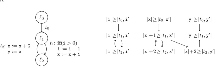
Fig. 5. Graph and RVG for the program of Ex. 4.10
To handle result variables α∈ (u\=). ∩C that add a constant dα, we consider how
often this addition is performed. Thus, while TimeBounds from Thm. 3.6 uses the size
approximationS to improve the runtime approximationR,SizeBoundsusesRto improveS.
For each transitiont∈ T, letCt=C∩ {|t, v0| |v∈ V} be all result variables fromC that
use the transitiont. SinceR(t) is a bound on the number of times thatt is executed, the
repeated traversal oftincreases the overall size by at mostR(t)·max{dα|α∈(u\
.
=)∩Ct}.
Example 4.9. Consider the result variableα=|t1,y0|in the RVG of Fig. 4. Its local size
bound is Sl(t1,y0) =|y|+ 1, i.e., each traversal oft1increasesybydα= 1. As before, we
use the size bounds on the predecessors of the SCC{α} as a basis. The input value when
entering this (non-trivial) SCC is S(t0,y0) = 0. Since t1 is executed at most R(t1) =|x|
times, we obtain the global bound S(α) =S(t0,y0) +R(α)·dα= 0 +|x| ·1 =|x|.
If the SCCCuses several different transitions from (u\=), then the effects resulting from.
these transitions have to beadded, i.e., the repeated traversal of these transitions increases
the overall size by at mostP
t∈T(R(t)·max{dα|α∈(u\
.
=)∩Ct}). Note that we use the
same size bound for all result variables of an SCC, since the transitions in an SCC may
influence all its result variables. So for an SCCCwhere all result variables are in the classes
.
= oru, we obtain the following new size bound for all result variables ofC:
max({S( ˜α)| there is anα∈Cwith ˜α∈pre(α)\C} ∪ {cα|α∈
.
=∩C})
+P
t∈T(R(t)·max{dα|α∈(u\
.
=)∩Ct})
Example 4.10. As an example for a program with several transitions that add constants, consider the program in Fig. 5. We are interested in determining a bound for the SCC
C={|t1,x0|,|t2,x0|}, and assume thatR(t1) =R(t2) =|i|has already been inferred. Using
Thm. 4.6, we obtainS(t0,x0) =|x|. Then, we can derive:
S(t1,x0) = S(t2,x0) =
max{S(t0,x0)}+ X
t∈T(R(t)·max{dα|α∈(u\
.
=)∩Ct})
=max{|x|}+ (R(t1)·max{1}) + (R(t2)·max{2})
=|x|+ (|i| ·1) + (|i| ·2)
=|x|+ 3· |i|
This bound is also used for the variableythat is modified in the same loop of the program.
The reason is that for the trivial SCC{|t2,y0|}of the RVG, by Thm. 4.6 we haveS(t2,y0) = Sl(t2,y0) (S(t1,i0),S(t1,x0),S(t1,y0)). AsSl(t2,y0) =|x|+ 2 andS(t1,x0) =|x|+ 3· |i|, we
`0
`1
`2
t0
t1:if(i>0) i:=i−1
x:=x+i
t2:if(i≤0)
[image:14.612.141.458.98.206.2]t3:if(x>0) x:=x−1
|i| ≥ |t0,i0| |x| ≥ |t0,x0|
|i| ≥ |t1,i0| |x|+|i| ≥ |t1,x0|
|i| ≥ |t2,i0| |x| ≥ |t2,x0|
|i| ≥ |t3,i0| |x| ≥ |t3,x0|
Fig. 6. Graph and RVG for the second program of Fig. 1
Finally, we discuss how to handle result variablesα∈× \˙ uthat sum and scale up several
program variables. For any suchαin a non-trivial SCCCof the RVG, letVα={v˜| |˜t,˜v0| ∈
pre(α)∩C}be the set of those program variables ˜vfor which there is a result variable |˜t,˜v0|
in Cwith an edge to α. For non-trivial SCCsC, we always haveVα6=∅. We first consider
the case where the scaling factor is sα = 1 and where|Vα|= 1 holds, i.e., where no two
result variables|ˆt,ˆv0|,|˜t,˜v0|inα’s SCCC with ˆv6= ˜v have edges toα. However, there may
be incoming edges from arbitrary result variablesoutside the SCC. Then,αmay sum up
several program variables, but onlyone of them comes fromα’s own SCCCin the RVG.
For each variablev, letfvαbe an upper bound on the size of those result variables|˜t, v0|∈/C that have edges to α, i.e.,fvα = max{S(˜t, v0)| |˜t, v0| ∈ pre(α)\C}. The execution of α’s transitiontthen means that the value of the variable inVαcan be increased by addingfvα(for allv∈actV(Sl(α))\Vα) plus the constanteα. Again, this can be repeated at mostR(t) times. The overall size is bounded by addingR(t)·max{eα+P
v∈actV(Sl(α))\Vαf
α
v |α∈( ˙×\u)∩Ct}.
Example 4.11. Consider the second program of Fig. 1 from Ex. 1.1 again. Its program
graph and RVG are depicted in Fig. 6. Our method detects the runtime boundsR(t0) = 1,
R(t1) =|i|, andR(t2) = 1. To obtain size bounds, we first infer the global size bounds
S(t,i0) =|i|for allt∈ T andS(t0,x0) =|x|. Next we regard the result variableα=|t1,x0|
with the local boundSl(α) =|x|+|i|. Thus, we haveα∈× \˙ u.
As α=|t1,x0| is a predecessor of itself and its SCC contains no other result variables,
we haveVα={x}. Of course,αalso has predecessors of the form|t,˜i0| outside the SCC.
We have actV(Sl(α)) = actV(|x|+|i|) = {i,x}, and fiα = max{S(t0,i0),S(t1,i0)} =
|i|. When entering α’s SCC, the input is bounded by the preceding transitions, i.e., by
max{S(t0,i0),S(t1,i0),S(t0,x0)}= max{|i|,|x|}. By traversingα’s transitiont1 repeatedly
(at most R(t1) = |i| times), this value may be increased by addingR(t1)·(eα+fiα) =
|i| ·(0 +|i|) =|i|2. Hence, we obtainS(α) = max{|i|,|x|}+|i|2. Consequently, we also get S(t2,x0) =S(t3,x0) = max{|i|,|x|}+|i|2.
From the inferred size bounds we can now derive a runtime bound for the last transition
t3. When we callTimeBoundsonT0={t3}, it finds the PRFPol(`2) =x, implying thatT0’s
runtime is linear. When program execution reaches T0, the size ofxis bounded byS(t2,x0).
SoR(t3) =R(t2)·[Pol(`2)](S(t2,i0),S(t2,x0)) = 1· S(t2,x0) = max{|i|,|x|}+|i|2. Thus, a
bound on the overall runtime isP
t∈TR(t) = 2 +|i|+ max{|i|,|x|}+|i|2, i.e., it is linear
in |x|and quadratic in|i|.
While the global size bound for the result variable|t1,x0| ∈× \˙ uin the above example is
only quadratic, in general the resulting global size bounds for result variablesαfrom the
class ˙×can be exponential. This is the case when the scaling factorsαis greater than 1 or
`0
`1
`2
t0
t1:if(i>0) i:=i−1 x:=x+y y:=x
[image:15.612.115.487.90.202.2]t2:x:=x+y y:=2·x
|i| ≥ |t0,i0| |x| ≥ |t0,x0| |y| ≥ |t0,y0|
|i| ≥ |t1,i0| |x|+|y| ≥ |t1,x0| |x|+|y| ≥ |t1,y0|
|i| ≥ |t2,i0| |x|+|y| ≥ |t2,x0| 2·(|x|+|y|)≥ |t2,y0|
Fig. 7. Graph and RVG for the program of Ex. 4.14
Example 4.12. To illustrate that, consider the following loop.
while z>0 dox:=x+y;y:=x;z:=z−1;done
Here, we have a transition t1= (`1, τ1, `1) whereτ1is the formula z>0∧x0 =x+y∧y0 = x0∧z0 = z−1. For αx =|t1,x0| andαy =|t1,y0| we obtain Sl(αx) = Sl(αy) = |x|+|y|.
Thus,αx andαy together form an SCC C where Vαx =Vαy ={x,y}. In other words, in
each iteration of the loop, the value of xandyis not increased by a fixed value as before
(that is not modified itself in the loop), but the value ofxandy is doubled in each loop
iteration. The reason is that here we have |Vαx|=|Vαy|= 2.
In general, each execution of a transition t may multiply the value of a result variable
from ( ˙× \u)∩Ct by max{|Vα| | α ∈ ( ˙× \u)∩Ct}. Since this multiplication may be
performed R(t) times, the repeated traversal of t increases the overall size by at most
(max{|Vα| |α∈( ˙× \u)∩Ct})R(t).
If the SCCCuses several different transitions ( ˙× \u), then the effects resulting from these
transitions have to bemultiplied. Thus, the overall increase is bounded by a multiplication
with the following exponential factor.
s×˙ = Y
t∈T (max{|Vα| |α∈( ˙× \u)∩Ct}) R(t)
In Ex. 4.12, ( ˙× \u)∩Ct is empty for all transitionst exceptt1. As |Vαx|=|Vαy|= 2 andR(t1) =|z|, we haves×˙ = 2|z|which results in the global size boundsS(αx) =S(αy) = 2|z|·max{|x|,|y|}.
Example 4.13. In Ex. 4.12, the exponential growth of the size was due to|Vαx|=|Vαy|> 1. A similar effect is obtained if one has scaling factorssα>1. To demonstrate this, consider the following modification of the above loop.
while z>0 dox:= 2·x;z:=z−1;done
Now the resulting transition t1 has the formula z >0∧x0 = 2·x∧z0 =z−1 and for
αx = |t1,x0| we obtain Sl(αx) = 2· |x|. In each iteration of the loop, the value of x is multiplied by the scaling factor sαx= 2.
To capture this, we revise the definition ofs×˙ as follows.
s×˙ = Y
t∈T
max{sα|α∈( ˙× \u)∩Ct} · max{|Vα| |α∈( ˙× \u)∩Ct}
R(t)
Then the overall increase is again bounded by a multiplication with an exponential factor. Similar to Ex. 4.12, in Ex. 4.13 we haves×˙ = (sαx· |Vαx|)
R(t1)= (2·1)|z|= 2|z|which results
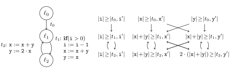
Example 4.14. As an example for a program with several transitions that
corre-spond to scaled sums, consider the program in Fig. 7. Its RVG has an SCC C =
{|t1,x0|,|t2,x0|,|t1,y0|,|t2,y0|} where all results variable are in ˙× \u. We can easily
de-rive S(t0,x0) = |x|, S(t0,y0) = |y| with Thm. 4.6, and deduce R(t1) = R(t2) =|i|. We
observe that s|t2,y0| = 2, and that the scaling factor is 1 for all other result variables.
Moreover, we have|Vα|= 2 for allα∈C. For our SCC, we then computes×˙ as follows:
s×˙ =
max{s|t1,x0|, s|t1,y0|} ·max{|V|t1,x0||,|V|t1,y0||} R(t1)
·max{s|t2,x0|, s|t2,y0|} ·max{|V|t2,x0||,|V|t2,y0||} R(t2)
=max{1,1} ·max{2,2}|i|·max{1,2} ·max{2,2}|i|
= 2|i|·4|i|= 8|i|
Intuitively, this means that the inputs to the SCCC can grow at most by a factor of 8|i|.
As no constants are added in the SCC, we can then compute the size bound on all result variables ofC ass×˙ ·max{S(t0,x0),S(t0,y0)}= 8|i|·max{|x|,|y|}.
Thm. 4.15 extends the procedureSizeBoundsfrom Thm. 4.6 to non-trivial SCCs. Note
that if an SCC contains a result variableβ whose local size bound does not belong to any
of our three classes, then we are not able to derive any global size bounds (i.e., then Thm.
4.15 cannot improve the current size approximationS). This is the case whenβ /∈×˙ (since
.
=⊆u⊆×˙).
Theorem4.15 (SizeBounds for Non-Trivial SCCs). Let(R,S)be a complexity
ap-proximation,Sl a local size approximation, and C⊆RV a non-trivial SCC of the RVG. If
there is aβ ∈C withβ /∈×˙, then we setS0 =S. Otherwise, for all β /∈C letS0(β) =S(β). For all β∈C, we setS0(β) =
s×˙ ·
max({S( ˜α)| there is anα∈C with α˜ ∈pre(α)\C} ∪ {cα|α∈
.
=∩C})
+P
t∈T(R(t)·max{dα|α∈(u\
.
=)∩Ct})
+P
t∈T(R(t)·max{eα+Pv∈actV(Sl(α))\Vαf
α
v |α∈( ˙× \u)∩Ct})
.
ThenSizeBounds(R,S, C) =S0 is also a size approximation.
Taking a different perspective, one can see our contributions on the inference of size bounds as a technique for computing potentially non-linear invariants. Our technique also takes runtime complexity analysis results into account, and its automation requires only relatively benign linear constraint solving in most cases.
5. HANDLING RECURSION
Our representation of programs as sets of simple transitions is restricted to programs without procedure calls. Of course, as long as there is no recursion (or only tail recursion), procedure calls can easily be “inlined”. However, in Sect. 5.1 we present an extension of our approach to handle arbitrary (possibly non-tail recursive) procedure calls. Based on this, we show in Sect. 5.2 how to adapt PRFs in order to infer exponential runtime bounds for recursive programs.
5.1. Complexity Analysis for Recursive Programs
Example 5.1. As an example, regard the following program where the recursive procedure
int facSum(int x)
`0:r:= 0
`1:whilex≥0 do
`2: r:=r+fac(x) | {z }
`3
x:=x−1
done
`4:returnr
int fac(int x)
`5:r:= 1
`6:ifx>0 then
`7: r:=x·fac(x−1) | {z }
`8
fi
`9:returnr
We extend the notion oftransitions to the form (`, τ,P), whereP is a non-empty multiset
of locations. If P is a singleton set {`0}, we write (`, τ, `0) instead of (`, τ,{`0}). By using transitions with several target locations, we can express function calls, since one target location represents the evaluation of the called function, whereas the other target location represents the context which is executed when returning from the function call. Thus, the program from Ex. 5.1 can be represented by the following transitions. Note that our transitions are an over-approximation of the original program since we do not take the
results of procedure calls into account (i.e., the value of the variable r0 is arbitrary in the
transitionst3 andt8).
t0 = (`0, x0=x∧r0= 0, `1)
t1 = (`1, x≥0∧x0 =x∧r0=r, {`2, `3})
t2 = (`1, x<0∧x0 =x∧r0=r, `4)
t3 = (`2, x≥0∧x0 =x−1, `1)
t4 = (`3, x0=x, `5)
t5 = (`5, x0=x∧r0= 1, `6)
t6 = (`6, x>0∧x0 =x∧r0=r, {`7, `8})
t7 = (`6, x≤0∧x0 =x∧r0=r, `9)
t8 = (`7, x0=x, `9)
t9 = (`8, x>0∧x0 =x−1, `5)
Aconfiguration is now amultiset of pairs (`,v) of a location`and a valuationv:V →Z.
Anevaluation step takes a pair (`,v) in the current configuration and applies a transition to it.7So for a configurationF, we writeF →t(`,v)F0for anevaluation stepwith a transitiont= (`, τ,{`1, . . . , `k})∈ T iff there is a pair (`,v)∈F,F0 = (F\{(`,v)})∪{(`1,v0), . . . ,(`k,v0)},
and the valuations v, v0 satisfy the formula τ. To ease readability, sometimes we write
→t instead of→
(`,v)
t . Note that in each evaluation step we only evaluate one pair in the
configuration (i.e., this does not model concurrency where several pairs are evaluated in parallel). So in Ex. 5.1, we have
{(`0,v0)} → (`0,v0)
t0 {(`1,v1)} →
(`1,v1) t1
{(`2,v1),(`3,v1)} → (`2,v1)
t3 {(`1,v2),(`3,v1)} →
(`3,v1) t4
{(`1,v2),(`5,v3)} → (`5,v3) t5 . . .
for v0(x) = v1(x) = v3(x) = 2, v2(x) = 1, v0(r) = 3, v1(r) = 0, v2(r) = −17, and
v3(r) = 42.
Obviously, such an evaluation can also be represented as anevaluation tree whose nodes
have the form (`,v). IfF→(t`,v)F0 as above, then in the corresponding evaluation tree, the node (`,v) has the children (`1,v0), . . . ,(`k,v0), and the edges to the children are labeled
(`0,v0)
(`1,v1)
(`2,v1)
(`1,v2)
(`3,v1)
(`5,v3)
. . .
t0
t1 t1
t3 t4
t5
witht. So the evaluation above would be represented by the tree
on the right. Albert et al. [2011a] and Debray et al. [1997] propose a similar notion of evaluation trees or computation trees for cost relations.
Note that for termination and for size complexity analysis, one could also replace transitions with multiple target locations like (`1, τ,{`2, `3}) by the corresponding single-target transitions
(`1, τ, `2) and (`1, τ, `3). But for runtime complexity analysis, this
is not possible. The reason is that the transition (`1, τ,{`2, `3})
means that evaluation continues both at location `2 and at
lo-cation `3. Hence, the runtime complexities resulting from these
two locations have to be added to obtain a bound for the runtime
complexity resulting from location`1. In contrast, the two transitions (`1, τ, `2) and (`1, τ, `3)
would mean that evaluation continueseither at location `2 or at location `3. Hence, here
it would suffice to take themaximum of the runtime complexities resulting from`2and`3
to obtain a bound for the runtime complexity resulting from`1. For example, the program
{t0, . . . , t9}above has quadratic runtime complexity. But if one replaced the transitiont1by
two separate transitions from`1to`2and from `1 to`3, then the resulting program would
only have linear runtime complexity.
By adapting the required notions in a straightforward way, our approach for complexity analysis can easily be extended to programs with (possibly recursive) procedure calls. As
before, theruntime complexity rc maps sizesmof program variables to the maximal number
of evaluation steps that are possible from a start configuration (`0,v) withv≤m. The only
change compared to Def. 2.3 is that configurations are now multisets of pairs (`,v):
rc(m) = sup{k∈N| ∃v0, F .v0≤m∧ {(`0,v0)} →k F}.
Similarly,runtime approximationsRfrom Def. 2.4 also have to be adapted to the new notion
of configurations. Now,Ris aruntime approximation iff the following holds for allt∈ T:
(R(t))(m)≥sup{k∈N| ∃v0, F .v0≤m∧ {(`0,v0)}(→∗◦ →t)kF}
As in Def. 2.6, the definition ofsize approximations S must ensure thatS(t, v0) is a bound
on the size of the variablev after a certain transitiont was used in an evaluation. However,
we now regard transitionst of the form (`, τ,P) whereP is a multiset of locations. Thus, we
require that whenever there is an evaluation from an initial configuration to a configuration
F such thattcan be applied for the next evaluation step (i.e., such that (`,v)∈F andv,v0
satisfyτ for some valuationsv andv0), thenS(t, v0) must be a bound for |v0(v)|. In other
words,S is asize approximation iff for all (`, τ,P)∈ T and allv∈ V, we have
(S((`, τ,P), v0))(m)≥sup{|v0(v)| | ∃v
0, F,v,v0. v0≤m ∧ {(`0,v0)} →∗F∧
(`,v)∈F ∧ v,v0 satisfyτ}.
Similarly, Slis a local size approximation iff
(Sl((`, τ,P), v0))(m)≥sup{|v0(v)| | ∃v,v0.v ≤m∧v,v0 satisfyτ}.
To denote the transitions that may precede each other, we also have to adapt the definition
of “pre” (which is needed for the computation of size approximations in Sect. 4). Here, we
have to take into account that a transition may reach a subsequent transition multiple times. Therefore, we now definepre((`0, τ0,P0)) to be the multiset where (`, τ,P)∈ T is contained
ktimes inpre((`0, τ0,P0)) iff`0 is containedktimes inP and there existv0, F,v,v0,v00 such
that {(`0,v0)} →∗F, (`,v)∈F, v,v0 satisfyτ, andv0,v00satisfyτ0.
Finally, we also have to modify the notion of PRFs. We now measure composed config-urations {(`1,v1), . . . ,(`k,vk)} bysumming up the measures of their components (`i,vi).
one decreases it. As before, our goal is to use a PRF to deduce a bound on the runtime complexity. To this end, we have to ensure that the measure of a configuration is at least as large as the number of decreasing transition steps that can be used when starting the program evaluation in this configuration. However, this would not be guaranteed anymore for composed configurations, since the measures of their components can also be negative.
Therefore, when measuring a composed configuration ofk >1 components, we only sum up
those components with non-negative measure. This gives rise to the following definition.
Definition5.2 (PRF for Recursive Programs). We call Pol : L →Z[v1, . . . , vn] a PRF
forT iff there is a non-emptyT ⊆ T such that the following conditions hold:
— for all (`, τ,{`1, . . . , `k})∈ T, we have
— τ⇒(Pol(`))(v1, . . . , vn)≥(Pol(`1))(v10, . . . , v0n), ifk= 1
— τ⇒(Pol(`))(v1, . . . , vn)≥Pj∈{1,...,k} max{0,(Pol(`j))(v10, . . . , vn0)}, ifk >1 — for all (`, τ,{`1, . . . , `k})∈ T, we have
— τ⇒(Pol(`))(v1, . . . , vn)>(Pol(`1))(v10, . . . , v0n), ifk= 1
— τ⇒(Pol(`))(v1, . . . , vn)>Pj∈{1,...,k} max{0,(Pol(`j))(v10, . . . , vn0)}, ifk >1 — τ⇒(Pol(`))(v1, . . . , vn)≥1
With this definition of PRFs, the procedureTimeBoundsfrom Thm. 3.6 can also be used
for the new extended notion of programsT. For this, we now let the transitionsT` leading
to the location` be a multiset that contains all transitions (˜`,˜τ ,P)∈ T \ T0 with`∈ P. Here (˜`,˜τ ,P) has the same multiplicity in T` as the multiplicity of ` in P (i.e., if ` is containedktimes in P then (˜`,˜τ ,P) is containedktimes inT`). This is needed, because
the sub-program T0 is reached k times by the transition (˜`,τ ,˜ P). Moreover, we now set
L0 = {` | T` 6=∅ ∧ ∃ P0.(`, τ,P0) ∈ T0} as entry locations. With this extension of our
method, for the program of Ex. 5.1 (with the initial location `0) we obtain the runtime
approximationsR(t3) =|x|(for the loop offacSum) andR(t9) =|x|+|x|2 (for the linear
recursion of facthat is called linearly often fromfacSum). The overall runtime bound is
P
t∈TR(t) = 8 + 12· |x|+ 5· |x|2, i.e., the program’s runtime is quadratic in the size of x.
Alonso-Blas et al. [2013] propose a technique to obtain runtime bounds in closed form by
means of sparse cost relations as an approximation for the overall cost of a cost relation.
Their technique allows to consider cost relations with more than one target location and, at the same time, only count the cost resulting from a single equation in each step. This is similar to Def. 5.2 where we also only count the number of evaluation steps of the transitions
in T instead of having to count all transitions in a single proof step.
5.2. Exponential Complexities for Recursive Programs
We consider two sources for exponential runtime complexity: (1) a variable takes a value of exponential size or (2) non-linear recursion. We handled the former in Sect. 4 by deriving exponential size approximations from polynomial runtime approximations. However, up to
now adirect application of polynomial ranking functions (that does not rely on size bounds
computed for preceding loops) could only yield polynomial runtime bounds. We now adapt and extend a technique by Albert et al. [2011a] to use polynomial ranking functions in order to infer exponential bounds for recursive programs directly (Case (2)). In contrast to the approach by Albert et al. [2011a], our adaptation allows to infer exponential complexity
bounds for onlysome of the transitions and polynomial bounds for others.
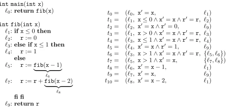
Example 5.3. Our technique works for recursive algorithms with multiple recursive calls, such as the (na¨ıve) recursive computation of the Fibonacci numbers. An implementation as an imperative program and its transitions are given in Fig. 8. Since we require that
int main(int x)
`0:returnfib(x)
int fib(int x)
`1:ifx≤0 then
`2: r:= 0
`3:else ifx≤1then
`4: r:= 1 else
`5: r:=fib(x−1) | {z }
`6
`7: r:=r+fib(x−2) | {z }
`8
fi fi
`9:returnr
t0= (`0, x0=x, `1)
t1= (`1, x≤0∧x0=x∧r0 =r, `2)
t2= (`2, x0=x∧r0 = 0, `9)
t3= (`1, x>0∧x0=x∧r0 =r, `3)
t4= (`3, x≤1∧x0=x∧r0 =r, `4)
t5= (`4, x0=x∧r0 = 1, `9)
t6= (`3, x>1∧x0=x∧r0 =r, {`5, `6})
t7= (`5, x>1∧x0=x, {`7, `8})
t8= (`6, x0=x−1, `1)
t9= (`7, x0=x, `9)
t10= (`8, x0=x−2, `1)
Fig. 8. Computation of the Fibonacci numbers with non-polynomial complexity
function that calls the recursive functionfib. Ast6 andt7 can occur Ω(fib(|x|)) times in
an evaluation of T (i.e., anexponential number of times), there does not exist any PRF
witht6∈ T or t7∈ T. The size of xremains bounded by its initial size throughout the
execution. Thus, the super-polynomial runtime cannot be inferred using the exponential size approximations from Sect. 4.
In Sect. 5.1, we discussed why we cannot just replace transitions with multiple target locations like (`3, τ,{`5, `6}) by the corresponding single-target transitions (`3, τ, `5) and
(`3, τ, `6) to infer polynomial bounds. However,exponential bounds can be inferred in this
way. Recall that Def. 5.2 required that the ranking function decreases over the sum of
all components of a configuration whenever a transition fromT is used. To weaken this
requirement, we now only require that the ranking function decreases in each individual
component. Then, in each path of the evaluation tree, the number ofT-edges is bounded
by [Pol(`0)], i.e., [Pol(`0)] is a bound for theheight h of the evaluation tree (if one only
countsT-edges to determine this height). For Ex. 5.3, this allows to infer the following
ranking functionPol:
Pol(`0) =Pol(`1) =Pol(`2) =Pol(`3) =Pol(`4) =x+ 2 Pol(`5) =Pol(`6) =x+ 1 Pol(`7) =Pol(`8) =Pol(`9) =x
In the constraints for the ranking functionPol, we have “separated” the transitiont6
into two transitions (from`3 to`5 and from `3 to`6). Similarly, t7 is separated into the
transitions from`5 to`7 and from`5 to`8. With the above ranking function Pol for the
“separated” version ofT, the transitionst6 andt7are inT (i.e., their separated versions
are strictly decreasing and they are bounded from below by 1). All other transitions are
weakly decreasing with the ranking functionPol.
When considering ranking functions separately for the different target locations of a
transition, we speak ofSeparated Ranking Functions (SRFs). To obtain complexity bounds
using SRFs, we have to find a bound on the number of evaluation steps with transitions from
T in the whole tree (i.e., not just in a single path of the tree). Note that each evaluation
step of the program corresponds to the step from an inner node toall of its children. Thus,
we have to approximate the number of inner nodes of the evaluation tree (and not the number
of its edges), because each inner node may haveseveral outgoing edges that correspond to
[image:20.612.125.489.92.265.2]