The Stability Cone for a Matrix Delay Difference Equation

(1)

Volume 2011, Article ID 860326,15pages doi:10.1155/2011/860326

Research Article

The Stability Cone for a Matrix Delay

Difference Equation

M. M. Kipnis

1

_{and V. V. Malygina}

2

1_{Department of Mathematics, South Ural State University, Chelyabinsk 454080, Russia}

2_{Department of Applied Mathematics and Mechanics, Perm State Technical University,}

Perm 614990, Russia

Correspondence should be addressed to M. M. Kipnis,[email protected]

Received 22 December 2010; Accepted 20 March 2011

Academic Editor: Frank Werner

Copyrightq2011 M. M. Kipnis and V. V. Malygina. This is an open access article distributed under the Creative Commons Attribution License, which permits unrestricted use, distribution, and reproduction in any medium, provided the original work is properly cited.

We construct a stability cone, which allows us to analyze the stability of the matrix delay diﬀerence equationxn Axn−1Bxn−k. We assume thatAandBarem×msimultaneously triangularizable

matrices. We constructmpoints inÊ

3_{which are functions of eigenvalues of matrices}_A_,_B_such

that the equation is asymptotically stable if and only if all the points lie inside the stability cone.

1. Introduction

Parameters of linear systems are subject to time changes. That is why in order to construct such systems it is desirable to know if they are not only stable but also able to estimate the distance of the system from the boundary of the stability region in the parameter space. Therefore, it makes sense to investigate the geometry of the subset of stable polynomials

in the space of characteristic polynomials of linear systems in the canonical space 1.

This idea has already been applied to the investigation of geometry of the subset of stable

polynomials in a two-dimensional subspace of the canonical space2,3, the stability simplex

for general diﬀerence equations4, connections of the convexity of the coeﬃcients sequence

with stability of diﬀerence equations5, and stability ovals for matrix diﬀerence equations

of the formxnxn−1Bxn−kwith the delayk6.

Consider the matrix equation

xnAxn−1Bxn−k, n0,1,2. . ., 1.1

wherek ∈ is the delay. Equations of the form1.1have been used for investigations of

(2)

solution of1.1with commutative matricesA, Band nonsingularAis given in9. But9

does not solve the stability problems of1.1. The stability of1.1was investigated in7,8,

10,11with special 2×2 matricesA, B. In12, the stability of1.1was investigated without

any restriction on the dimension but with the special matrixAαI,α∈, 0 α 1, where

Iis the identity matrix.

In this paper we give a geometric solution to the problem of asymptotic stability of

1.1in any dimension with simultaneously triangularizable matricesA, B. It is known that

commuting matrices are simultaneously triangularizable13. As usual, we say that1.1is

stable if its zero solution is stable. Our solution is based on constructing the stability ovals which, in turn, form a stability cone. At the same time we give an algorithm for checking the stability of the scalar equation

xnaxn−1bxn−k, n0,1,2. . . 1.2

with complex coeﬃcientsa, b.

The paper is organized as follows. In the second section, we recall the results on the

stability of the scalar equation1.2with real nonnegativeaand any realb14,15. Further

in that section we construct the stability oval for1.2with real nonnegative coeﬃcientaand

complex coeﬃcientb. In Section3, we consider a wider class of equations of the form1.2

witha, bbeing complex numbers. In Section4, we state a system of inequalities allowing us

to check the stability of the scalar equation1.2with two complex coeﬃcients. In Section5,

we give a geometrical criterion for the asymptotic stability of matrix equation 1.1 with

simultaneously triangularizable matrices. Besides, we establish nongeometric necessary and

suﬃcient conditions for the stability of matrix equation 1.1 in terms of inequalities. In

Section6, we use the stability ovals and cones for analysis of some numerical examples.

2. The Stability Oval for

1.2 with Real Nonnegative

a

and Complex

b

We start by stating the results from14,15in the form which is suitable for us. Since the case

k1 is obvious, we consider only the casek >1.

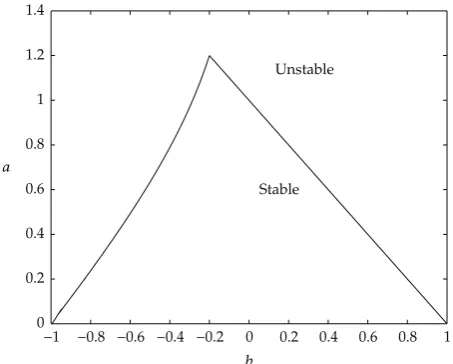
Theorem 2.1see14,15. In1.2letaandbbe real,a0,k >1.

1Ifak/k−1, then1.2is unstable.

2If 0 a < k/k−1, then1.2is asymptotically stable if and only if

−a2₁₋_2a_cos_ω

1< b <1−a, 2.1

whereω1 ∈0, π/kis the root of the equation

a sinkω

sink−1ω. 2.2

(3)

−1 −0.8 −0.6 −0.4 −0.2 0 0.2 0.4 0.6 0.8 1 0

0.2 0.4 0.6 0.8 1 1.2 1.4

a

b

[image:3.600.186.413.97.279.2]

Stable Unstable

Figure 1: The domain of asymptotic stability of1.2,a 0,k6.

Our first new result about the case of nonnegative realaand complexbin1.2is the

following.

Theorem 2.2. Leta0 be a real number andba complex number,k >1.

1Ifak/k−1, then1.2is unstable.

2If 0 a < k/k−1, then1.2is asymptotically stable if and only ifblies inside the oval

bounded by

bexpikω−aexpik−1ω, −ω1 ω ω1, 2.3

whereω1 ∈0, π/kis the root of2.2.

3If 0 a < k/k−1andbis outside of the stability oval2.3, then1.2is unstable.

4If 0 a < k/k−1andblies on the boundary2.3of the stability oval, then1.2is

stable (nonasymptotically).

Proof. We will use the D-decomposition method parameter plane method 16, 17. A

characteristic polynomial for1.2is the following:

fz zk₋_azk−1₋_b. _2.4

For any fixed value ofa, the complex plane of the parameterbis divided into some regions

by a curvefexpiω 0, that is,

(4)

Hence,D-decomposition occurs in the plane of the complex parameterbby means of a curve

bω expikω−aexpik−1ω, −π ω π. 2.6

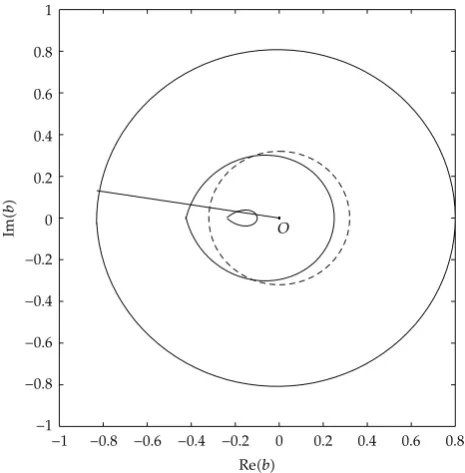
The example of theD-decomposition fork 6,a0.7 is shown in Figure2. From2.6we

obtain

|bω|2₁_a2₋_2a_cos_ω. _2.7

Therefore, |b| increases monotonically when ω runs from 0 to π. Similarly, |b| increases

monotonically whenωruns from 0 to−π. Let us construct an increasing sequenceωiri0of

all valuesω∈0, π, such that Imbωi Imb−ωi 0. Here 1 r k,ω0 0,ωr π.

Each pair of the curves2.6formed by motionωon intervalsωi, ωi1,−ωi1,−ωicreates a

new region ofD-decomposition of the complex plane of parameterb. This region necessarily

contains some real values ofbas the function|bω|is monotone on0, πand on−π,0. Due

to the properties of the regions, if some inner point of this region is an asymptotically stable

point, then the whole region consists of asymptotically stable points. Ifak/k−1, then

according to Theorem2.1there are no stable points on the axis Imb 0. Hence, there are no

stable points on the complex plane of parameterb. Let nowa < k/k−1. Letω1 ∈0, π/k

be the root of 2.2. Then the unique D-decomposition region containing the real straight

line segment2.1is the oval with the boundary2.3. Parts 1–3 of Theorem2.2are proved.

Direct checking shows that the derivative of a characteristic polynomial2.4is not equal to

zero on the boundary of the stability oval. Therefore, when the parameterbruns along the

boundary of the stability oval, all the corresponding roots zof the characteristic equation,

satisfying |z| 1, are simple. Hence, 1.2 is stable nonasymptotically. Theorem 2.2 is

proved.

Example 2.3. Letk6 and, also,1a0.2,2a0.75, and3a1.1. Letb0.33 expiα,

0 α <2π. Let us analyze the asymptotic behavior of the solutions of1.2for all values of

α. We construct three stability ovals for three values ofaand also the circleb0.33 expiα

Figure3. Theorem2.2and Figure3give the following result.1Fora 0.2, the equation

is asymptotically stable for any value ofα.2Fora 0.75, the equation is asymptotically

stable for 2.0918∼ α0 < α < 2π −α0 ∼ 4.1914, it is unstable forα /∈ α0,2π−α0, and it is

stablenonasymptoticallyforαα0andα2π−α0.3Finally, fora1.1, the equation is

unstable for any value ofα.

Example 2.4. Let k 6 and, also, 1 a 0.2, 2 a 0.75, and 3 a 1.1. Let b

rexpi19π/20, r 0. Let us find the asymptotic behavior of 1.2 for all values of r.

We construct the beam b rexpi19π/20together with three stability ovals Figure3.

Theorem2.2and Figure3give the following result.

1For a 0.2, the equation is asymptotically stable for 0 r < r1 ∼ 0.8276, it is

unstable forr > r1, and it is stablenonasymptoticallyforr r1.

2For a 0.75, the equation is asymptotically stable for 0 r < r2 ∼ 0.4080, it is

unstable forr > r2, and it is stablenonasymptoticallyforr r2.

3Finally, fora 1.1, the equation is stable for 0.1063∼ r31 < r < r32 ∼ 0.1944, it is

(5)

−2 −1.5 −1 −0.5 0 0.5 1 1.5 2 −2

−1.5 −1 −0.5 0 0.5 1 1.5 2

Im

(

b

)

Re(b)

[image:5.600.185.415.98.281.2]

O

Figure 2:D-decomposition of the complex plane of the parameterbfork6,a0.7.

Im

(

b

)

Re(b) O

−1 −0.8 −0.6 −0.4 −0.2 0 0.2 0.4 0.6 0.8 −1

−0.8 −0.6 −0.4 −0.2 0 0.2 0.4 0.6 0.8 1

Figure 3: Stability ovals fork 6, a 0.2, anda 0.75; a 1.1. A circleb 0.33 expiαand a beam

brexpi19π/20are constructed for Examples2.3and2.4.

3. The Stability Cone for

1.2 with Complex Coefficients

The family of stability ovals depending ona∈ k/k−1forms a surface which we call the

stability cone.

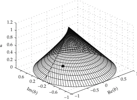
Definition 3.1. The stability cone for delay k is a surface in a three-dimensional space

Reb,Imb, zwith 0 z k/k−1, such that its intersection with any planez a0

[image:5.600.183.416.319.556.2]

(6)

−1 −1 −0.6

−0.2 0.2 0.6 0 0.2 0.4 0.6 0.8 1 1.2

−0.5 0

0.5 1

a

Im₍_b

[image:6.600.186.412.99.265.2]

) Re(b)

Figure 4: Stability cone fork6. The point on the cone is constructed for Example3.3.

The stability cone is the image of the two-dimensional domain in the spaceω, a

0 a sinkω

sink−1ω,

−π_k ω π

k

3.1

under the mapping into

3 _{by the functions}

Reb coskω−acosk−1ω,

Imb sinkω−asink−1ω,

za.

3.2

The stability cone fork6 is presented in Figure4.

Let us now study the problem of the stability of scalar equation1.2with complex

coeﬃcientsa, b. We consider the equation

xnρ1expiα1xn−1ρ2expiα2xn−k, 3.3

with real nonnegativeρ1, ρ2and realα1,α2. We setxnynexpinα1. Then3.3becomes

ynρ1yn−1ρ2expiα2−kα1yn−k. 3.4

Obviously,3.4is stableasymptotically stableif and only if3.3is stableasymptotically

stable. The stability problem of3.4can be solved due to Theorem2.2. Thus, we obtain the

(7)

Theorem 3.2. Consider3.3. Put

aρ1, bρ2expiα2−kα1. 3.5

Construct the pointM Reb,Imb, ain

3_.

1Equation3.3is asymptotically stable if and only if the pointMlies inside the cone3.2

(ifa0 andReb2 Imb2 <1, then the pointMis assumed to be the inner point

of the cone).

2If the pointMlies outside the cone3.2or on its top Reb −1/k−1, Imb

0, ak/k−1, then3.3is unstable.

3If the pointMlies on the boundary of a cone3.2, but not on its top, then3.3is stable

(nonasymptotically).

Example 3.3. Let us test the stability of the equation with complex coeﬃcients

xnσexp

_iπ

5

x_n−10.7 exp

_iπ

3

x_n−k 3.6

with a real parameterσand a delayk6. Put firstσ0. By Theorem3.2, according to3.5

we calculate

b0.7 expiπ

3 −6·

π 5

0.7 expi17π

15

. 3.7

The vertical lineReb,Imb, σ,0 σ <∞in

3 _{intersects the boundary of the stability}

cone atzσ0∼0.3442Figure4. To study the negative values ofσwe rewrite3.6:

xn−σexp

_i6π

5

x_n−10.7 exp

_iπ

3

x_n−k. 3.8

By Theorem3.2, according to3.5we calculate

b0.7 exp

i

_π

3 −6·

6π 5 0.7 exp _i17π 15 . 3.9

As the results3.9,3.7coincide, we obtain the following answer: 3.6is asymptotically

stable for−σ0< σ < σ0∼0.3442, and it is unstable forσ /∈−σ0, σ0. According to part 2 of

Theorem3.2forσσ0orσ−σ0,3.6is stablenonasymptotically.

Example 3.4. We test3.6with a real parameterσfor stability. Unlike the previous example

let now the delay be odd:k7. For positiveσby Theorem3.2, according to3.5we obtain

b0.7 exp

i

_π

3 −7·

(8)

The vertical lineReb,Imb, σin

3 _{intersects the boundary of the stability cone at}_z

σ0∼0.3377. To study the negative values ofσsimilarly to the previous example, we obtain

b0.7 expiπ

3 −7·

6π 5

0.7 expi29π

15

. 3.11

The results3.10,3.11do not coincide. For3.11the vertical lineReb,Imb, σ,0 σ <

∞intersects the boundary of the stability cone atz σ1 ∼0.3002. We obtain the following

answer:3.6withk 7 is asymptotically stable if−0.3002∼ −σ1 < σ < σ0 ∼ 0.3377, it is

unstable ifσ /∈−σ1, σ0, and it is stablenonasymptoticallyforσσ0orσ−σ1.

Comparison of Examples3.3and3.4reveals the diﬀerence in the behavior of3.3for

even and odd values of the delayk. Let us compare the stability of1.1and the following

equations:

xn−Axn−1Bxn−k, 3.12

xn−Axn−1−Bxn−k. 3.13

Substitutingxn −1nynreduces1.1to

yn −Ayn−1 −1kByn−k. 3.14

Equations 1.1 and 3.14 are simultaneously stable or unstable. Therefore, we have the

following symmetry property of the stability region for1.1.

Theorem 3.5. For even delayskthe (asymptotic) stability of 1.1implies the (asymptotic) stability

of3.12and vice versa. For oddkthe (asymptotic) stability of1.1implies the (asymptotic) stability

of3.13and vice versa.

Similar properties of symmetry have been specified in11,15for the scalar equation

1.2with reala, b.

4. A System of Inequalities for Checking the Stability of

3.3

In the previous sections we used some geometric procedures. In this section we construct

a system of inequalities in order to check the stability of 3.3. Henceforth we assume 0

argz<2πfor a complex variablez.

Theorem 4.1.

1Ifρ1 <1−ρ2, then3.3is asymptotically stable.

2If 1−ρ2 ρ1 < min1ρ2, k/k−1, then for the asymptotic stability of 3.3it is

necessary and suﬃcient to fulfill simultaneously the following conditionsH1,H2:

ρ2<

ρ2

(9)

whereω1∈0, π/kis the root of the equation

ρ1

sinkω

sink−1ω,

π−argexpiα2−kα1< π−k−1arccos

1ρ2

1−ρ22

2ρ1 −arccos

1−ρ2

1−ρ22

2ρ1ρ2 .

H2

3Ifρ1 min1ρ2, k/k−1, then3.3is not asymptotically stable.

Proof. The stability of3.3is equivalent to the stability of3.4, so we will work with3.4.

1Forρ1<1−ρ2by Theorem2.2the stability oval exists and the circle of radiusρ2lies

completely inside the oval. Therefore, Theorem2.2implies the asymptotic stability

of3.4. Part 1 of Theorem is proved.

2Let 1−ρ2 ρ1 <min1æ2,k/k−1. Let us consider two cases.

Case 11−ρ2 ρ1<1. In this case, the stability oval exists by Theorem2.2, and the origin

of the coordinates lies inside the oval. For3.4to be asymptotically stable, it is necessary and

suﬃcient to satisfy the two following conditions. The first one is that the circle of radiusρ2

should intersect the stability oval. It is equivalent toH1. The second condition is that the

argument of a point expiα2−kα1should be between the arguments of the two crosspoints

M1, M2of a circle of radiusρ2with the stability oval2.3. Let us assume that ImM1> 0,

and let the parameterωcorrespond to the pointM1. We obtain

argM1 argexpikω−ρ1expik−1ω

k−1ωargexpiω−ρ1

4.1

from2.3. But we also obtain

cosω 1ρ

2

1−ρ22

2ρ1

4.2

from2.7. Equalities4.1,4.2give

argM1 k−1arccos1ρ21−ρ22

2ρ1

arccos1−ρ

2

1−ρ22

2ρ1ρ2

. 4.3

It follows from4.3that the second requirement is equivalent toH2. Part 2 of Theorem4.1

is proved in Case1.

Case 21 ρ1<min1ρ2, k/k−1. By virtue of the inequalityρ1< k/k−1, the stability

oval exists, and, sinceρ11, the origin does not lie inside the oval. The same requirements as

in the previous case lead to the same conditionsH1,H2. Part 2 of the Theorem is proved.

3Letρ1min1ρ2, k/k−1. We consider two cases.

Case 1 1 ρ2 ρ1 < k/k −1. In this case the stability oval exists by Theorem 2.2,

and, by virtue of the inequality ρ1 1, the origin does not lie inside the oval. Due to the

inequalityρ2 ρ1−1, no point of the circle of radiusρ2lies inside the oval and so3.4is not

(10)

Case 2ρ1k/k−1. In this case,3.4is unstable by Theorem2.2.

Theorem4.1is proved.

As we see, the text of Theorem4.1does not contain any geometric terms. However,

Theorem 3.2has a considerable advantage over Theorem4.1because of its simplicity and

geometric visualization. That is why in the future examples we prefer describing the stability

of matrix equation1.1in geometric terms.

5. The Stability Cone for the Matrix Equation with Simultaneously

Triangularizable Matrices

In this section we consider1.1with simultaneously triangularizable matricesA,B.

Theorem 5.1. LetA, B, S∈

m×m _and_S−1_AS_A_T_and_S−1_BS_B_{T, where}_A_T_{, B}_T _{are the lower}

triangular matrices with elements, respectively,λjs, μjs1 j, s m. Let

bjμjjexpiargμjj−kargλjj, ajλjj 1 j m, 5.1

and let the pointsMjin

3 _{be constructed by}

MjRebj,Imbj, aj 1 j m. 5.2

Then1.1is asymptotically stable if and only if for anyj 1 j mthe pointMjlies inside cone

3.2.

If for somej 1 j mthe pointMjlies outside cone3.2, then1.1is unstable.

Proof. In1.1we substitutexn Synand multiply the equation byS−1. We obtain

ynATyn−1BTyn−k 5.3

with lower triangular matrices AT, BT. By virtue of the nondegeneracy of matrix S, the

stability of5.3is equivalent to the stability of1.1. Let us assume thatyn yn1, . . . , ynmT.

The system5.3consists ofmscalar equations

ynjλjjy_n−1j μjjy_n−kj

j−1

s1

λjsy_n−1s j−1

s1

μjsy_n−ks 1 j m. 5.4

As usual, 0_s₁ 0. Equation5.4is called exponentially stable if there are realC > 0, q ∈

0,1, such that for any solutionynjthe estimate

ynj Cqn max

−k u 1,1 s j

(11)

holds. The exponential stability is equivalent to the asymptotic stability for the equations under consideration. It is more convenient to prove the exponential stability. Let the points

5.2 1 j mlie inside the cone3.2. Due to Theorem3.2, all equations of the form

ynjλjjy_n−1j μjjy_n−kj 1 j m 5.6

are exponentially stable. Let us prove by induction onj that5.4are exponentially stable.

Forj 1,5.4coincides with5.6, so it is exponentially stable. Let, for anyr < j,5.4with

rinstead ofjbe exponentially stable. Then5.4is represented in the form

ynjλjjy_n−1j μjjy_n−kj gnj, 5.7

where|gnj|has an estimate of the form5.5by the induction assumption. Assuming zn

ynj, y_n−1j, . . . , y_n−kj T, we represent5.7in the form

znGzn−1hn, 5.8

whereG∈

k×k_,_G_{is a stable matrix, and}_|hn|_{has an estimate of the form}_{5.5. From}_5.8_we

obtainznGnz0 n_r₁Gn−rhr, which implies the exponential stability of5.4. The induction

is finished, and asymptotic stability of1.1is proved.

Let us assume that some point5.2does not lie strictly inside the cone. Then, for the

initial data in5.4, we assume thaty_−ns0 for anys, n, such that 1 s j, 1 n k. Thus,

5.4becomes5.6. If the point5.2lies on the cone boundary, then5.6has a trajectory

which does not tend to zero because the characteristic polynomial of5.6has a rootzsuch

that|z| 1. If some point5.2lies outside the cone, then by Theorem3.2the equation has

unlimited trajectories. Theorem5.1is proved.

Remark 5.2. If no points5.2lie outside the stability cone, but some of them lie on the cone

boundary, then1.1can be stablenonasymptoticallyor unstable.

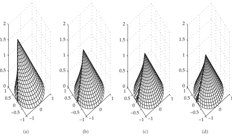
Remark 5.3. The stability conesFigure5are constructed for each delaykindependently of

the dimensionmin1.1. Ifk → ∞, then the intersection of all stability cones is the right

circular cone with the base radius 1 and the height 1. The interior of this cone is the “absolute stability domain,” that is, the stability domain for any delay.

The next theorem, which is the evident consequence of Theorems 4.1 and 5.1, will

establish the asymptotic stability criterion in the form of inequalities for matrix equation1.1.

Theorem 5.4. LetA, B, S∈

m×m _and_S−1_AS_AT_and_S−1_BS_{BT, where}_{AT, BT} _{are the lower}

triangular matrices with elementsλjs, μjs 1 j, s m, respectively. Let

(12)

−1 −1 0 1 0.5 1.5 2

−0.5 0 0

1

0.5 1

a −1 −1 0 1 0.5 1.5 2

−0.5 0 0

1

0.5 1

b −1 −1 0 1 0.5 1.5 2

−0.5 0 0

1

0.5 1

c −1 −1 0 1 0.5 1.5 2

−0.5 0 0

1

0.5 1

[image:12.600.113.485.94.313.2]

d Figure 5: Stability cones fork2,3,4,5.

Construct a setAS⊆P {j∈ : 1 j m}by the following rules (cf. Theorem4.1).

1Ifρ1j<1−ρ2j, thenj ∈AS.

2If 1−ρ2j ρ1j<min1ρ2j, k/k−1, then forj∈ASit is necessary and suﬃcient to

fulfill simultaneously the following conditionsH1j,H2j:

ρ2j<

ρ2

1j1−2ρ1jcosω1j, H1j

whereω1j∈0, π/kis the root of the equation

ρ1j sinkω

sink−1ω,

_π₋_arg

expiα2j−kα1j< π−k−1arccos1ρ

2

1j−ρ22j

2ρ1j −arccos

1−ρ2

1j−ρ22j

2ρ1jρ2j .

H2j

3Ifρ1jmin1ρ2j, k/k−1, thenj /∈AS.

Equation1.1is asymptotically stable if and only ifASP.

6. Examples of the Stability Oval and the Cone for Matrix Equations

Example 6.1. Consider the equation

(13)

−0.6 −0.4 −0.2 0 0.2 0.4 0.6 0.8 1 −0.6

−0.4 −0.2 0 0.2 0.4 0.6 0.8

Im

(

b

)

[image:13.600.185.415.98.280.2]

Re(b)

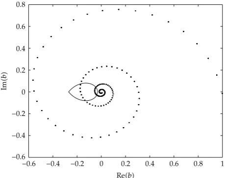
Figure 6: The stability oval and pointsMs_{for Example}_6.1_.

where

A

cosα −sinα

sinα cosα

, B

cosβ −sinβ

sinβ cosβ

6.2

withα0.0314,β0.1745. Let us find out for what values ofs∈ 6.1is stable. Matrices

A, Bare commuting; therefore, they are simultaneously triangularizable. The eigenvalues of

matricesA, Bareλ1,2 exp±0.0314iandμ1,2 exp±0.1745icorrespondingly. In Figure6

the stability oval is shown, which is the section of the stability cone3.2on the levelz

1.0309. By Theorem5.1we have to know whether the points

Ms _0.9680s_cos_0.1745s₋_0.1884,_0.9680s_sin_0.1745s₋_0.1884 _6.3

lie inside the cone. Figure6illustrates that pointsMs enter the oval of stability twices

53, s87and leave it twices58, s94. The conclusion is that the system6.1,6.2is

stable for 53 s 58 and for 87 s 94 and is unstable for all the other values ofs.

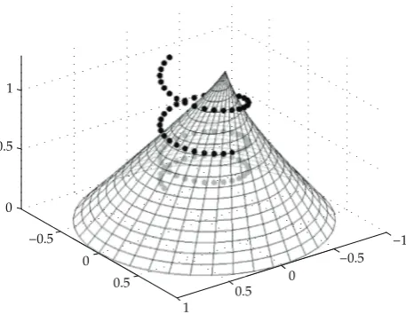
Example 6.2. Consider the equation

xn 1

3A

s_xn−1_Axn−6, _6.4

where

A

0 1.0150

−1.0150 2.0300

(14)

−1 −0.5 0

0.5 1

−0.5 0 0

0.5

[image:14.600.186.415.103.280.2]

0.5 1

Figure 7: The stability cone and pointsMs_{for Example}_6.2_{. Grey points}_Ms₁

s 49are located

inside the cone therefore6.4is stable. Dark pointsMss 50are located outside therefore 6.4is unstable.

Let us find out for what values of s ∈ 6.4 is stable. The eigenvalues of Aare

λ1,2 1.0150 exp±0.0374i. Stability ovals are symmetric about the real axis. Therefore, by

Theorem5.1, only points

Ms_{0.3383 cos0.03741}₋_6s,_{0.3383 sin0.03741}₋_6s,1.0150s

3

6.6

see Figure7should be checked. Figure7displays that pointsMsfor 1 s 49 are inside

the stability cone3.2and fors50 points are outside of the stability cone. The conclusion

is that6.4is stable for 1 s 49 and it is unstable fors50.

7. Conclusion

The stability analysis for1.1in

m _{can be reduced to the pole placement problem for a}

polynomial of degreekm. Our geometric approach allows us to reduce the dimension. To use

the approach, we need to know the eigenvalues of A, B. This is the problem of finding the

roots of a polynomial of degreem. Using these eigenvalues, we get a finite sequence of points

in

3 _{such that their position with respect to the stability cone allows us to make a conclusion}

about the stability of1.1.

In our future work we intend to analyze the stability of equationxn Axn−mBxn−k

with two delaysm, kwith simultaneously triangularizable matricesA, B. The scalar version

of this equation was examined in 2, 3, 18. The stability cone for the matrix diﬀerential

equation ˙xt Axt Bxt−τwas introduced in19.

Acknowledgment

(15)

References

1 A. T. Fam and J. S. Meditch, “A canonical parameter space for linear systems design,” IEEE

Transactions on Automatic Control, vol. 23, no. 3, pp. 454–458, 1978.

2 Y. P. Nikolaev, “The geometry of D-decomposition of a two-dimensional plane of arbitrary coeﬃcients of the characteristic polynomial of a discrete system,” Automation and Remote Control, vol. 65, no. 12, pp. 1904–1914, 2004.

3 M. M. Kipnis and R. M. Nigmatulin, “Stability of trinomial linear diﬀerence equations with two delays,” Automation and Remote Control, vol. 65, pp. 1710–1723, 2004.

4 M. M. Kipnis and D. A. Komissarova, “A note on explicit stability conditions for autonomous higher order diﬀerence equations,” Journal of Diﬀerence Equations and Applications, vol. 13, no. 5, pp. 457–461,

2007.

5 V. M. Gilyazev and M. M. Kipnis, “Convexity of a sequence of coeﬃcients and the stability of discrete systems,” Automation and Remote Control, vol. 70, pp. 1856–1861, 2009.

6 I. S. Levitskaya, “A note on the stability oval forxn1xnAxn−k,” Journal of Diﬀerence Equations and

Applications, vol. 11, no. 8, pp. 701–705, 2005.

7 S. Guo, X. Tang, and L. Huang, “Stability and bifurcation in a discrete system of two neurons with delays,” Nonlinear Analysis: Real World Applications, vol. 9, no. 4, pp. 1323–1335, 2008.

8 E. Kaslik and S. Balint, “Bifurcation analysis for a two-dimensional delayed discrete-time Hopfield neural network,” Chaos, Solitons & Fractals, vol. 34, no. 4, pp. 1245–1253, 2007.

9 J. Dibl´ık and D. Y. Khusainov, “Representation of solutions of discrete delayed systemxk1

AxkBxk−mfkwith commutative matrices,” Journal of Mathematical Analysis and Applications, vol. 318, no. 1, pp. 63–76, 2006.

10 H. Matsunaga, “Stability regions for a class of delay difference systems,” in Differences and Differential Equations, vol. 42 of Fields Institute Communications, pp. 273–283, American Mathematical Society,

Providence, RI, USA, 2004.

11 H. Matsunaga and C. Hajiri, “Exact stability sets for a linear diﬀerence system with diagonal delay,”

Journal of Mathematical Analysis and Applications, vol. 369, no. 2, pp. 616–622, 2010.

12 E. Kaslik, “Stability results for a class of diﬀerence systems with delay,” Advances in Diﬀerence Equations, vol. 2009, Article ID 938492, 13 pages, 2009.

13 R. Horn and C. Johnson, Matrix Theory, Cambridge University Press, Cambrige, UK, 1986.

14 S. A. Kuruklis, “The asymptotic stability ofxn1−axn bxn−k 0,” Journal of Mathematical

Analysis and Applications, vol. 188, no. 3, pp. 719–731, 1994.

15 V. G. Papanicolaou, “On the asymptotic stability of a class of linear diﬀerence equations,” Mathematics

Magazine, vol. 69, no. 1, pp. 34–43, 1996.

16 E. N. Gryazina and B. T. Polyak, “Stability regions in the parameter space: D-decomposition revisited,” Automatica, vol. 42, no. 1, pp. 13–26, 2006.

17 D. D. ˇSiljak, “Parameter space methods for robust control design: a guided tour,” IEEE Transactions on

Automatic Control, vol. 34, no. 7, pp. 674–688, 1989.

18 F. M. Dannan, “The asymptotic stability ofxnK axn bxn−1 0,” Journal of Diﬀerence Equations and Applications, vol. 10, no. 6, pp. 589–599, 2004.

(16)

Submit your manuscripts at

http://www.hindawi.com

Hindawi Publishing Corporation

http://www.hindawi.com Volume 2014

Mathematics

Journal of

http://www.hindawi.com Volume 2014 in Engineering

Hindawi Publishing Corporation http://www.hindawi.com

Differential Equations

International Journal of

Volume 2014

Applied MathematicsJournal of

Probability and Statistics Hindawi Publishing Corporation

http://www.hindawi.com Volume 2014 Journal of

Mathematical PhysicsAdvances in

Complex Analysis

Journal of

Optimization

Journal of Hindawi Publishing Corporation

Combinatorics

International Journal of

http://www.hindawi.com Volume 2014 Operations Research

Journal of

Function Spaces

Abstract and Applied Analysis Hindawi Publishing Corporation

International Journal of Mathematics and Mathematical Sciences

Hindawi Publishing Corporation http://www.hindawi.com Volume 2014

The Scientific

World Journal

Algebra

Discrete Dynamics in Nature and Society

Decision Sciences

Discrete Mathematics

Journal of

The Stability Cone for a Matrix Delay Difference Equation

Research Article