Theoretical and Experimental Analysis of a Coupled System Proportional Control Valve and Hydraulic Cylinder

Theoretical and Experimental Analysis of a Coupled

System Proportional Control

Valve and Hydraulic Cylinder

R. Amirante

_{, A. Lippolis , P. Tamburrano}

Polytechnic University of Bari, Italy, tel. +39 080 5963470 – amirante@poliba.it *Corresponding Author: amirante@poliba.it

Copyright © 2013 Horizon Research Publishing All rights reserved.

Abstract

system actuated by a proportional directional control valve on a hydraulic cylinder. In order to evaluate the dynamic interaction between the proportional valve and the cylinder theoretical analysis, numerical simulations as well as experimental test are performed. Coupling cylinder and proportional valve, it is very important to know the ratio of their natural frequencies. In particular, if the valve is characterized by a lower natural frequency, its behavior prevails so that no resonance peak can be observed on the coupled system. On the contrary, resonance phenomena can be observed in all the other cases. It is important that these phenomena are preventively taken into account to realize a precise and accurate control system of a hydraulic axle.At last, three different control methods are tested on the coupled system:Proportional Integral Derivative technique (PID), the adaptive “One-Step-Ahead” control technique, and an expert control technique and the obtained precisions are very interesting.

Keywords

Control Valve, Linear Hydraulic Actuator

1. Introduction

The hydraulic axes practice has become very wide-spread in many applications. Usually hydraulic axes are more flexible than classical axes with ball-screw electrically-controlled, and also they can produce strong accelerations. The main difficulty is the physical system control, just because the hydraulic systems are very not linear.

Usually a high dynamics of proportional valve means a high quality control for a closed loop system hydraulically driven, but this opinion can be deceptive.

Many research papers propose interesting and effective modelling and analysis of proportional

valves[1][2][3][4][5][6][7]. However, to the authors’ knowledge, there are not many studies dealing with analysis of the dynamic interaction between a proportional valve and a linear actuator.The importance to analyse the whole system (the proportional valve and controlled hydraulic cylinder) is underlined in this paper. The Authors focus the attention to evaluate the dynamic interaction between a proportional valve and a synchronous cylinder and then the consequent control system performed by a closed loop control on hydraulic system characterized by a differential cylinder controlled by a proportional directional control valve.

suitable for experimental applications in which the system is a black box controlled by a closed loop. This technique has shown good performances in controlling of hydraulic transmission tested in a previous paper[3].

2. Theoretical Analysis

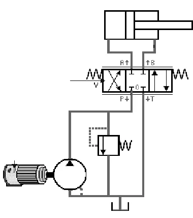
In the following, the hydraulic system behaviour is analysed;it consists of a differential cylinder driven by a proportional valve (fig.1).In order to describe the dynamics of the directional proportional valve spool, the valve behaviour is approximated by a second order system. This approximation could be considered acceptable; only the hypothesis that the damping effects are proportional to velocity is not accurate but opportune in order to simplify the model. The characteristic curves, concerning some directional proportional valves, underlines that the most of commercial valves have a near critical damping coefficient value.

Figure 1. Hydraulic system, cylinder and valve

The relationship between the flow rate and the electrical signal applied to obtain valve opening is very complex and due to:

 a) the relationship between the spool displacement and opening area: in particular, a linear function (e.g. rectangular opening area) simplifies the control system, while parabolic function or, in general, not linear function allows a better control at low flow rates;

 b) “the lap”: when the electrical signal is near to zero, the behaviour of the valve is strongly dependent on this parameter. There are commercial valve with high dynamic performances, called “zero lap”, these valves, usually, are characterized by a tolerance, between spool and sleeve edges, near to ±0,5% in relation to the total spool stroke. In this case, theoretically, there is not discontinuity between electrical signal and flow rate near to zero; but, really, a discontinuity between these parameters always exists because the tolerance above reported cannot be preserved, due to pilot edge wear in time. It is

important to underline that these valves (zero lap) are in the minority, usually under lap valve are used for position control, in order to obtain the best

promptness,while overlap valves are used for velocity controls, these valves are able to reduce internal leakage improving the hydraulic seal in normal position (corresponding to zero electrical signal).

 c) the relationship between the valve pressure drop and the flow rate is not linear.Moreover, hysteresis, repeatability and inversion error make more complex the control and are conditioned by electrical driving method [1][2].

The cylinder system is doubtless more complex than valve system. In this case the hydraulic fluid, with its compressibility, is the elastic element of the system, while damper effect is due to different causes: friction between piston and cylinder, internal leakage and, principally, the opening behaviour of the proportional valve. To explain the last effect, the free oscillations of cylinder piston can be analysed. For ease, a synchronous cylinder (left piston area equal to right piston area) with the same capacity volume V in both chambers (included the volume of the pipe) is considered (fig. 2).

Figure 2. Directional proportional valve and hydraulic cylinder The behaviour of a proportional directional control valve is simulated by a throttle on both connections P→A and B→T (again fig. 2). The forces equilibrium of cylinder can be written[20,21]:

(1) where p1 and p2 are the pressures in the two cylinder

chambers, A is the piston area, M is the whole mass of the piston included the connected elements moved by cylinder,xis the piston displacement, t the time.

The compressibility law of the hydraulic fluid, with reference to left and right cylinder chambers, is:

and (2)

2 2 2

1 )

(

t x M A p p

∂ ∂ = −

V V E

p 1

1

∆ = ∆

V V E

p 2

2

where E is equivalent (fluid and pipe) bulk module. The time derivative of above written equations is:

and

(3) where Qt1and Qt2represent the external leakage crossing the left and right throat orifice area of the directional proportional valve when the connection among the valve ports are P→A and B→T. Usually, flow behaviour in the hydraulic valves is turbulent[5], but in order to simplify the calculations and to obtain a linear equation, the flow behaviour is supposed laminar and then can be written[20,21]::

and (4)

where K is an appropriate proportional constant depending on the valve opening, whilep10 and p20are pressures upstream the valve (fig. 2).

Replacing eqs. 4 ineqs. 3, these expressions can be written:

(5)

(6)

Deriving (1) regards to time and adding it the same eqn. 1 multiplied by an appropriate constant, the following equation is obtained:

(7) after some simple arithmetical operations, the second order equation of the piston velocity c can be obtained:

(8)

The eqn. 8 is the classical equation of a second order dynamics system, in which is the angular frequency and the damper factor ζ is:

(9)

In these formulas, to simplify the analytic treatment, some approximations have been considered: right cylinder and pipe volume is equal to left one, the valve metering sections are the same and consequently K constants are the same for

both connections (P→A and B→T), the flow rate trough

throttles has been considered laminar.

The analytic result above reported could be physically explained: when the spool is in neutral position and so every valve connection is closed, if the piston is submitted to an initial displacement from equilibrium condition and let it to oscillate free, the piston would transform alternatively elastic energy (depending on compressibility of the hydraulic fluid) into kinetic energy of piston and vice versa. On the contrary, when the valve is open or the leakage trough the valve is not negligible, elastic energy is dampened by the throttles presence.

The proportional directional control valve acts like the throttles above described, in fact the volumetric flow (through the same valve) can be ideally divided into two components: the first is the steady component and takes into account of the valve opening conditions and valve supply pressure, while the second takes into account the volumetric flow rate oscillations due to pressure oscillations. This last one has a dampening effect, in fact when pressure level rises (and consequently kinetic energy grows) this one induces a volumetric flow rate reduction through the valve similar to throttles leakage.

The cylinder system, in the most common practical applications, acts like an under dampened system, which has strong resonance overshoots near to natural angular frequency ωn: for examples, the damper factor value calculated by eqn. 9 for used experimental device is equal to

0,2. The damper factor is function of valve operating conditions (coefficient K in eqn. 9) and it is not a characteristic of cylinder but it is time dependent: the damper factor is very close to zero when the valve is near the neutral position, instead it increases when the valve is open. Using simple formulations and some approximations, it is demonstrable [20]that dampening effects due to friction and internal leakage in cylinder system are negligible in comparison to the dampening effects due to directional control valve.

To understand the cylinder-valve system behaviour and to optimize the control system, it is very important the knowledge of γparameter, defined as ratio between directional control valve natural frequency and cylinder natural frequency. With reference to γ parameter, it is possible to show four different situations[22]:

 a)γ<<1, it’s the most common case, in which the resonance peak of the cylinder is very reduced depending on the high damper value of regulation valve near to the cylinder natural frequency. In this case it’s suitable to use an high time derivative constant in a PID control system, to improve the regulation amplitude recovering the valve dampening effect.

 b) γ<1, in this case the valve natural frequency is       ₊ ∂ ∂ − = ∂ ∂ − = ∂ ∂ 1 1 1 t Q t x A V E t V V E t p       ₊ ∂ ∂ − − = ∂ ∂ − = ∂ ∂ 2 2 2 t Q t x A V E t V V E t p ) ( 0 1 1 1 K p p

Qt = − Qt2 =K (p2−p20)

0 1 1 1 0 1 1

1 _{( )}

p K V E t x V EA p K V E t p p p K V E t x V EA t p + ∂ ∂ − = + ∂ ∂ − − ∂ ∂ − = ∂ ∂ 0 2 2 2 0 2 2

2 _{( )}

p K V E t x V EA p K V E t p p p K V E t x V EA t p + ∂ ∂ + = + ∂ ∂ − − ∂ ∂ + = ∂ ∂

)

(

2

p

p

K

MV

EA

c

MV

EA

t

c

K

V

E

t

c

₊

₌

₋

∂

∂

+

∂

∂

ω

n 2 8

2

2 = 2 =

smaller than cylinder natural frequency and so the valve produces a little reduction of resonance amplitude due to the cylinder.In this case,itcan be not necessary to use the derivative component, while a proportional control, with a suitable gain, is enough.

 c) γ>1, the dampening power of the valve, close to the frequency in which the cylinder resonates, is not important, for this reason it is necessary choosing a control that allows a strong reduction of resonance phenomena. It is necessary to use a control with a first order time delay block(the so called PT1 block) [20], with limit frequency equal to 50% about the frequency of the cylinder.

 d) γ>>1, in this case the natural frequency of the regulation valve is greater than the resonance depending on the cylinder.This one is not dampened and also a PT1 control is useless, it is suitable using some controls able to produce artificial dampening effects, like that defined “State-Observer”.

In this paper only the case a) will be experimentally analysed. To schedule the experimental tests, a numerical simulation has been performed a priori by a commercial code named ITI-SIM. The code provides the possibility to model engineering system and in particular hydraulic plants. In fig. 3 the block diagram used to simulate the experimental plant is reported.

Figure 3. Numerical simulation block diagram

The ITI-SIM code uses the modeling by signal block diagrams: the cylinder block has intrinsically the possibility to fit the theoretical model above described. The valve block does not allow simulating the spool dynamics and spool position is considered algebraically depended to the valve input signal. However, every signal blocks (fig. 3) can be customized by use of macros to simulate particular systems. In this case the macros added to the valve can simulate the spool dynamics in according to second order system above illustrated. Numerical results have shown a good agreement with the performed experimental test, but for conciseness reasons, only an example will be presented in the following paragraphs.

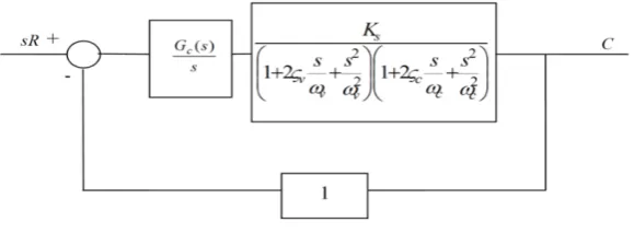
In the following, the system stability is theoretically analysed. Referring to a cylinder position control, the block

scheme equivalent to the experimental plant is presented in fig.4in the Laplace domain.

Figure 4. Control block scheme - position control where:

s is the Laplace variable,

R is the time depending target position,

C is the time depending actual piston velocity (controlled variable)

Gc(s)Transfer Function of controller,

is the transfer function of valve-cylinder system; in agreement with the model illustrated in previous section, both cylinder transfer function and valve transfer function is described by a second order system dynamics. Where ωc and ωvare the natural angular frequencies of cylinder and valve,

ζ_c and ζ_v are the respective damper factors and Ksis the proportional constant concerning valve-cylinder system. If the system was linear, Ks would be the piston velocity connected with a valve input signal equal to 1 Volt. Since the system is not linear, Ks must be interpreted as the derivative of the velocity as regards input signal, calculated with regard to the operative point.

According to the physical system, the controlled variable

C is the piston velocity; in fact, the valve input signal causes a valve spool displacement and so it fixes the volumetric flow rate across the valve, finally the piston velocity is proportional to the volumetric flow rate. The feedback signal is measured by means of a linear encoder, then the feedback variable is the piston position and the feedback transfer function is an integral type function, for this reason the valve-cylinder system is an intrinsic integrator system and so the integral effect can be neglected in the used control technique.

The previous block scheme (fig. 4) is referred to the position control, but this one is, theoretically, equivalent to the velocity control. In fact this scheme, using the reduction laws of block schemes, can be transformed in an equivalent scheme (fig. 5) with unitary feedback to represent velocity control scheme. In this case, the input variable is the derivative of piston displacement, or better piston velocity.So the control transfer function concerning to velocity control must be the integral of the control transfer function concerning position control.

Gc(s)

    

  

+ +     

  

+ +

2 2 2

2

2 1 2

1

c c c v v v

s

s s s s

K

ω ω ς ω ω

ς

s

1 -

+

R C













+

+













+

+

2

1

2

1

c c c v

v v

s

s

s

s

s

K

ω

ω

ς

ω

Figure 5. Control block scheme – velocity control

Referring to linearized block scheme shown in fig. 4, it’s possible to analyse the stability of the system using the Routh Criterion: supposing a proportional control Gc(s)=Kp, if γ is the ratio between ωv/ωc and replacing ωc with ω, the transfer function equivalent to closed loop system can be writtenas:

(10)

Imposing that there are not real positive roots, by the Routh Criterion, after simple calculations it can be observed:

 a) growing Kp, the valve-cylinder system becomes unstable,

 b) the most important parameter of stability control is the product of every constant on the direct and feedback line.In this case the product constant is

Kp⋅Ks . Particularly, it’s note worthy that the ratio of

Kp⋅Ksto the cylinder frequency ω depends on γratio.

 c) the stability.

Fig.6 shows the stability parameter Kp⋅Ks/ωas function of γ(assuming ζc = 0.05 and ζv = 0.9) with reference to the proportional control. Note thatthe stability parameter, initially, grows with the valve frequency (corresponding to γ

parameter for an assigned cylinder frequency).It arrives to a max value for γ=0.7 and then it decreases with valve frequency. This trend is explainable because the valve behaves like a low pass filter because of its natural frequency lower than cylinder one. Thus valves, with low natural frequency compared to cylinder frequency, need a proportional control with a high gain to reduce its damping effect. The stability of the system valve-cylinder grows with the natural frequency of the valve until its value becomes comparable with the cylinder one. In this case, the valve loses its dominant effects and a purely proportional control could increase cylinder oscillation near its resonance frequency.

The stability of the system is also analysed for different values of ωvtaking into account the valve-cylinder system root locus showed in fig. 7, both assuming ζv=0.7 and ζc=0.2

and considering a pure proportional control. The root locus is a powerful approach to analyse the stability and dynamic response of the system and it can show how changes in one of a system's parameters (typically is loop gain) will change the close-loop poles positions and thus change the system's dynamic performance. The poles of the closed loop characteristic are the roots of characteristic equation

1+KG(s)=0, where G(s) is the open-loop transfer function of the system, including the transfer function of the controller,

and K is the system gain. The system valve-cylinder has five poles (fig. 7): one pair of complex conjugate poles p1-p1’ relevant to the valve, one pair of complex conjugate poles p2-p2’ relevant to the cylinder and one pole p3 placed at the origin introduced to pass from a velocity control to a position control.

Figure 6. Proportional and proportional derivative control: stability limits

on γ variation

The valve poles are closest to the imaginary axis so they have the greatest influence on the closed-loop response. By the root locus, relevant to valve natural frequency fv = 20 Hz, it can be noticed that, growing the system loop gain, valve poles asymptotically head for infinity moving to right half-plane thus leading the system to instability. The cylinder poles, instead, asymptotically head for infinity staying on the left half-plane. It is evident, from root loci plotted for fv = 60 Hz and fv =85 Hz, that the stability of the system valve-cylinder grows with the natural frequency of the valve until its value becomes comparable with cylinder one. In this case, growing the loop gain, the cylinder poles asymptotically head for the right half-plane conditioning the stability of the system.

The same analysis can be carried out for the PD control. In this case Gc(s) = Kp (1+τd s) and the transfer function becomes:

p s c

v c

v c

v

s

e _{s s s s s K K}

s K s

G _{5 4 2 2 3} 2 4_{3 2 2 2 4 2 4}

) (

2 ) 1 4

( )

( 2 )

(

ω

γ

ω

γ

γ

ς

γ

ς

ω

ς

γς

γ

ω

ς

γ

ς

ω

ω

γ

+ +

+ +

+ +

+ +

(11)

The stability parameter KpKs/ωis function of time constant τd, or in particular of a dimensional time constant t=τdω. The same fig.6shows four curves relative, respectively, to values 0.5, 1, 2, 3 of a-dimensional time constant t of a PD control.

The diagrams analysis explains how for lowγ (valve natural frequency lower than cylinder natural frequency) the derivative component improves the dynamics of valve-cylinder system because it compensates the dampening effect of the valve and also it is opportune to stabilize the system. Vice versa, when γ grows, the derivative contribute produces a negative effect on stability of the system because it reduces max value of the stability parameter.

Figure 7. System valve-cylinder root loci for different value of ωv with ζc =0.2andζv =0.7 with reference to the P control

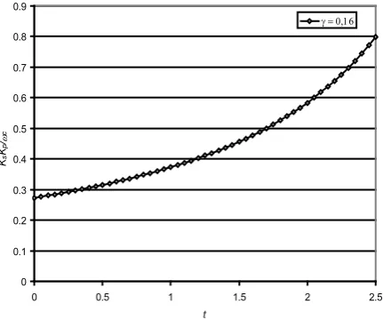
In the next fig.8 is reported the stability parameter as function of a dimensional time constant t=τ_dω,for an assigned value of γ = 0.16 equal to the experimental plant γvalue; it is evident the stabilising effect of derivative component.

Figure 8. Proportional and proportional derivative control: stability limits for the γ experimental value (0,16)

In fig. 9 a comparison between theoretical values and experimental values of Kp stability limit is shown. Again figure 9 (obtained for γ = 0.16) confirms the growing of system stability if the time derivative constant grows.

In fig. 10, the root locus considering a proportional derivative control, with Kp=1.5 and Kd=0.05, is shown. The PD controller introduces a real zero z1 and improves the stability of the system. The improvement of the stability, obviously, is confirmed by the higher value of the critical gain compared with the pure proportional controlled system one.

Figure 9. Experimental and theoretical values of proportional coefficient: stability limits

Figure 10. System valve-cylinder root locus with ζc =0.2 and ζv =0.7 with reference to the PD control

3. The Experimental Plant

To validate theoretical analysis and to perform experimental test, a test-rig has been realized at the Polytechnic University of Bari (Italy).

) 1 ( )

) (

2 ) 1 4

( )

( 2 (

) 1 ( )

( _{5 4 2 2 3 3 2 2 2 4 2 4}

4 2

s K

K s

s s

s s

s s K K s

G

d p s c

v c

v c

v

d p s

e _{ω ς γ ς ω γ γς ς ω ς γ ς γ γ ω γ ω τ}

ω γ τ

+ +

+ +

+ + +

+ + +

+ =

0 0.1 0.2 0.3 0.4 0.5 0.6 0.7 0.8 0.9

0 0.5 1 1.5 2 2.5

t

Ks Kp /cω

γ = 0,16

1.0 1.5 2.0 2.5 3.0 3.5 4.0 4.5 5.0

0.0 0.5 1.0 1.5 2.0 2.5

t

Kp

Figure 11. Layout of hydraulic system

The hydraulic scheme of circuit has been reported in fig. 11, and it is constituted by an hydraulic open circuit and in particular composed by:

 a 30 kW three-phase asynchronous electric motor. Its rotational speed can be regulated by means of an electrical inverter, within the range 0÷3000 rpm

according to the pump speed range.

 a gear pump (63 cm3_{) which supplies hydraulic} power. Its operation field is 700÷1500 rpm and its maximum working pressure is equal to 350 bar.

 a directly operated pressure relief valve; by

regulation of this valve, the pressure value of 80 bar on the feed line is established.

 a four-way proportional directional valve, with a y

(fig. 11) input signal range of -5 ÷+5 Volt. The valve has an overlap and when the input signal is in the range ±1 Volt the flow rate is always zero.

 a differential cylinder, with cylinder bore of 60 mm, stroke of 1 m, piston rod diameter of 40 mm and a moving mass of 13 kg.

 flexible pipes (1 inch internal diameter) connect all the components of the hydraulic circuit.

An automatic system based on Labview software is used to electronically monitor the behaviour of the hydraulic plant during the experimental tests.Such system is managed by a personal computer and a 16-bit acquisition card, which is characterized by a maximum sampling frequency of 1 MHz.This card manages 16 analogical acquisition channels, two analogical output channel, two digital counter, 16 digital input/output channels and two counters TTL compatible. An analogical output channels has been used to send input signal to the proportional valve. The control system period is approximately 0.1ms and it depends on the CPU type.

The cylinder piston displacement (the controlled variable) is measured using an optical linear encoder, which produces two TTL compatible signals with 90 shift phase degrees. The pitch, corresponding to each time base of square wave, is 8

µm. The TTL compatible signals of the linear encoder are acquired by the digital counter and also by the analogical channels to a post processing analysis.

The directional proportional valve displacement is driven by the analogical output signal of the data acquisition card, thus allowing a rapid increase or decrease of internal orifices area[1].

4. Results and Discussion

The first step has been to verify the dynamic performance of the proportional valve: the experimental test-rig cannot analyse the valve alone, but the whole valve-cylinder system.

Taking into account the cylinder geometry, the natural frequency is approximately80 Hz, while the natural frequency of the proportional directional valve is near to 20 Hz.The cylinder dynamics is negligible compared to the dynamics of the valve-cylinder system because the γ ratio is less than one.

Figure 12. Bode diagram, catalogue and experimental data referred to first only harmonica after a Fourier analysis

According to the proportional valve technical catalogue details, the experimental Bode-diagram (fig. 12) has been obtained using an electrical input signal equal to 50% of max input signal (5 Volt) added to a sinusoidal oscillation with a fixed amplitude equal to 5%of the max input signal. Fig. 13 shows the time history of velocity piston and electrical input signal. By the sinusoidal input signal at frequency of 2 Hz, the piston velocity time history (fig. 13, 14) shows strong oscillations around the sinusoidal law. These oscillations are not due to electrical noise or to numerical causes but they are mechanical oscillations depending on piston natural frequency. In fact the cylinder displacement is measured by means of a digital signal, so the background noise is not present, the only possible error is depending on the encoder resolution (8 μm). Moreover, acquiring the two output encoder signals by analogical channels it is possible to reach a 2 μm resolution, corresponding to 90 shift phase degrees, by a data post processing. The velocity measurement is obtained as a mean value on a 2 ms time interval, consequently the final error is approximately 1 mm/s.

-6.00 -5.00 -4.00 -3.00 -2.00 -1.00 0.00

1 10 frequency (Hz) 100

A

m

pl

itude (

db)

0 30 60 90 120 150

P

has

e (

deg.

)

amplitude catalog features -dump. factor 0,7 amplitude - experimental data

phase - experimental data

Figure 13. Cylinder velocity time history and valve input signal (2 Hz). On the contrary, the amplitude of velocity oscillations (fig. 14) is approximately 15 mm/s, one order greater than velocity error. This result confirms the measuring reliability and the mechanical nature of high frequency phenomena above reported.

The same error analysis can be carried out with time measurement reference: a 100 kSample/s analogical acquisition is performed on the two digital signal (TTL compatible) and, for this reason, the time measurement error is about 10 μs on 2ms time interval.Consequently, the velocity percentage error due to time measure is very low and equal to0,5%.

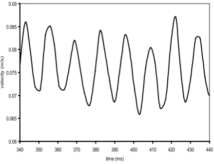
Figure 14. Cylinder velocity time history and valve input signal (16 Hz). Figure15 shows an enlargement of fig. 13to evaluate these oscillations.Note there are about 8 oscillations in a 100 ms

time interval, therefore the oscillation frequency is about 80 Hz. This experimental frequency value is in good agreement with the cylinder natural frequency computed by eqn. 8. This value can be theoretically evaluated only by an exact knowledge of fluid compressibility, pipes stiffness and connected volumes. In figure 1, two long pipes (about 1.5 m) between cylinder and valve are evident, in opposition with an efficient industrial application. Moreover, the presence of

these big connected volumes is finalized to approach the cylinder frequency to valve frequency, to underline the phenomena plotted in fig. 15. If the valve-cylinder system was linear, these oscillations could be dampened and the final output signal could be characterized by the same frequency of input signal. Vice versa, these oscillations persist because of non-linearity of the system. The amplitude of oscillations due to natural frequency of cylinder is comparable to the input signal amplitude and this effect introduces another noise to non-linearity of the system and in particular to the goodness of control.

Figure 15. An enlargement of cylinder velocity. The natural cylinder frequency (about 80 Hz) is shown

The time history of velocity piston and electrical input signal for a frequency input signal of 16 Hz is shown in fig. 14.

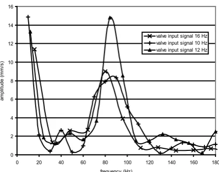
A Fourier analysis is applied to the piston velocity signal, and the greatest amplitude is found on the first harmonica.However, another amplitude peak is visible near the natural cylinder frequency (fig. 16). The experimental Bode-diagram, compared with catalogue data, is shown in fig. 12.

Note the velocity has the amplitude value of the first harmonica approximately equal to 20 mm/s,while the sinusoidal component amplitude of input signal is 0.25 Volt. Therefore the Ksvalue, introduced in Control Theoretical Aspects section, is 80 mm/sVolt.

The hydraulic cylinder natural angular frequency ωnis approximately equivalent to 500 rad/s and the stability parameter Kp⋅Ks/ω(fig, 8) for the proportional control, is equal to 0.27.Therefore the bigger Kp value to avoid the instability is 0.27⋅ 500/80 = 1.6 Volt/mm. This Kp value is near to the value experimentally obtained.

During the experimental test, the gear pump rotates ata constant velocity (1200 rpm), to be sure that the pressure relief valve is always open.Than the pressure on the proportional valve inlet port is 80 bar, fixed by the pressure relief valve.

To obtain an experimental value of the control coefficients, the position control tests are performed with many different

0.02 0.04 0.06 0.08 0.1 0.12 0.14

100 200 300 400 500 600 700 800 900 1000 time (ms)

ve

lo

ci

ty (

m

/s)

0 0.5 1 1.5 2 2.5 3

P

ropor

tional

S

ignal

(

V

ol

t)

Piston velocity Proportional signal

0.06 0.07 0.08 0.09 0.1 0.11 0.12 0.13 0.14 0.15

100 200 300 400 500 600 700 800 900 1000 time (ms)

ve

lo

ci

ty (

m

/s)

1 1.2 1.4 1.6 1.8 2 2.2 2.4 2.6 2.8 3

P

ropor

tional

s

ignal

(

V

ol

t)

Piston velocity Proprtional signal

0.06 0.065 0.07 0.075 0.08 0.085 0.09

340 350 360 370 380 390 400 410 420 430 440

time (ms)

ve

lo

ci

ty (

m

values of these coefficients.

Figure 16. Velocity amplitude spectral analysis at different valve signal input frequency

Figure 17. Cylinder position control by P technique, Kp = 1.1 and target

position 100 mm

Figure 17shows the piston time response with target position 100 mm by using a P control technique and

Kp=1.1.After a dead time of about 60ms, due to valve response time (about 40 ms) and hydraulic fluid compressibility, the piston reaches a constant velocity, compatible with the valve characteristic at the maximum input signal and then reaches the target position near to 1200 ms.Again figure17shows the absolute control error to evaluate the goodness of this kind of control. The displacement time history is not absolutely monotonic (a little overshoot is visible) but the final absolute error is very little (about 0.2 mm).

Growing the proportional coefficient, for example Kp=1.2, the little overshoot is more evident (fig.18). After this displacement overshoot, the cylinder changes its direction and then stops, with a final error about 0.15 mm.

Figure 18. Cylinder position control error, by P technique, Kp = 1.2 and

target position 100 mm.

In figure 19, the same kind of control is tested, but using a proportional coefficient Kp=1.6. The time history shows dampened oscillations around the target value. In figure 20 the system instability is evident and the piston oscillations have a frequency equal to 8 Hz, while the amplitude is approximately 6 mm. Note the proportional algorithm does not show a static error, because valve/cylinder system is an intrinsic integrator to control piston position. Consequently, an integral technique is not necessary in this application.

Figure 19. Cylinder position control, by P technique, Kp = 1.6 and target

position50 mm

To confirm the behaviour of the whole valve/cylinder system, a comparison between experimental and numerical data is shown in fig. 21 with Kp=2. The simulation scheme utilized is shown in fig. 3 and the behaviour of directional proportional valve is approximated by a second order system with natural frequency equal to 20 Hz and ζ=0.7. The comparison between experimental and numerical data is very good: the same frequency and amplitude values can be observed.

0 2 4 6 8 10 12 14 16

0 20 40 60 80 100 120 140 160 180 frequency (Hz)

am

pl

itude (

m

m

/s

)

valve input signal 16 Hz valve input signal 10 Hz valve input signal 12 Hz

0 20 40 60 80 100 120

0 500 1000 1500 2000 2500

time (ms)

di

spl

ac

em

ent

(m

m

)

-2 -1,5 -1 -0,5 0 0,5 1 1,5 2

erro

r (m

m

)

Piston position error (mm)

0 20 40 60 80 100 120

0 500 1000 1500 2000 2500

time (ms)

di

spl

ac

em

ent

(m

m

)

-2 -1.5 -1 -0.5 0 0.5 1 1.5 2

erro

r (m

m

)

Piston position error (mm)

0 10 20 30 40 50 60

0 200 400 600 800 1000 1200 1400 1600

time (ms)

di

spl

ac

em

ent

(m

m

)

-4 -3 -2 -1 0 1 2 3 4

erro

r (m

m

)

Figure 20. Cylinder position control, by P technique only (Kp=2.5) and

target position 100 mm.

Figure 21. Cylinder position control. A comparison instability control is shown between numerical plant simulation and experimental data (Kp=2).

Figure 22. Cylinder position control, by PD technique (Kp=1.5, Kd=0.05)

and target position 500 mm

In figure 22 the PD technique is applied on the hydraulic system. On the base of theoretical consideration reported on the previous paragraph, the use of differential parameter in the control technique allows increasing the proportional coefficient without producing instability.

In this figure, the time history of piston displacement and control error is shown. The control coefficient are: Kp=1.5

and Kd=0.05, while the target position is set to 500 mm. The output displacement (controlled variable) approaches very well the target position.

In the following the cylinder velocity control is tested. It is possible to set an appropriate law of piston velocity (fig.23),at the same of position control.

Figure 23. Target Cylinder velocity law.

The velocity control tests can be performed by many different kinds of regulation techniques. Three different control methods are considered:

a PID technique;

a close loop expert control technique;

an adaptive “One-Step-Ahead” control technique.

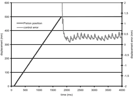
First, a proportional integral and differential control is used; in fig. 24 the theoretical and experimental time sequence of piston displacement, together with the displacement error, is shown.T he error grows initially very fast because of the dead time, due to valve response time and hydraulic fluid compressibility. Then the displacement error is approximately constant (approximately 1 mm) with exiguous oscillations. Finally, in the deceleration face, the time delay of the valve produces a recovery of the initial piston displacement error.

Figure 24. Cylinder velocity control by PID technique (Kp=10, Ki =1,5

Kd=0,05)

0 20 40 60 80 100 120

0 500 1000 1500 2000

time (ms)

di

spl

ac

em

ent

(m

m

)

-8 -6 -4 -2 0 2 4 6 8

erro

r (m

m

)

Piston position error (mm)

0 10 20 30 40 50 60

0 100 200 300 400 500 600 700 800 900 1000 time (ms)

Pi

st

on pos

ition (

m

m

)

Experimental data Numrical data

0 100 200 300 400 500 600

0 500 1000 1500 2000 2500 3000 3500 4000 time (ms)

di

spl

ac

em

ent

(m

m

)

-2 -1,5 -1 -0,5 0 0,5 1 1,5 2

di

spl

ac

em

ent

er

ror

(m

m

)

Piston position control error

0 0.02 0.04 0.06 0.08 0.1 0.12

0 100 200 300 400 500 600 700 800 900 1000

time (ms)

pi

st

on v

el

oc

ity

(

m

/s

)

0 10 20 30 40 50 60 70 80

0 200 400 600 800 1000 1200

time (ms)

di

spl

ac

em

ent

(m

m

)

-0.6 -0.4 -0.2 0 0.2 0.4 0.6 0.8 1 1.2 1.4

di

spl

ac

em

ent

er

ror

(m

m

)

In fig. 25 the time sequence of piston displacement is shown, obtained by use of an expert control technique in which an approximate law between piston velocity and electrical input signal is assigned based on the experimental valve-cylinder dynamics knowledge.

Figure 25. Cylinder velocity control by expert control technique based on the knowledge of valve-cylinder system characteristics (Kp=10, Ki =1,5

Kd=0,05).

To delete the little error obtained on this experimental control law, a closed loop is however adopted to improve the control quality by a PID technique. So the control error is less than 0.2 mm

Also, an adaptive control technique has been used. In particularly, the One-Step-Ahead adaptive control technique has been used.This technique is very powerful in the control of hydraulic transmission, as demonstrated in a previous paper[3].

Figure 26. Block layout of the One-Step-Ahead control technique. The One-Step-Ahead adaptive control technique combines a parameter estimation algorithm (fig. 26), with

the control scheme: the Least Squares algorithm will be used for an on-line estimation of the linearized model parameters on the basis of the previous sequence of the hydraulic system inputs and outputs. Then the control scheme will be applied to the linearized estimated model of the controlled system[18][3].

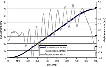
Figure 27 shows the velocity control system by using the One-Step-Ahead technique. In the acceleration phase the displacement error is sufficiently low because the algorithm is able to estimate very well the initial valve time delay. During the constant velocity phase, the control is not able to steady the calculation of estimator block and the error is notably fluctuating.

Figure 27. Cylinder velocity control by “One Step Ahead” technique.

5. Conclusions

This paper analysed the driving system actuated by a proportional directional control valve on an hydraulic cylinder. In order to evaluate the dynamic interaction between the proportional valve and the cylinder theoretical analysis, numerical simulations as well as experimental test were performed. The results demonstrated that the knowledge of interaction between the proportional valve and the cylinder was indispensable to optimize the design parameters. At beginning the dynamics of cylinder-valve system was analysed and the frequency response of this system was experimentally obtained. This analysis was very important just because all these phenomena were taken into account to realize an accurate control of a hydraulic axle. It was possible to observe that the piston velocity time history showed strong oscillations around a sinusoidal law and these oscillations were due to mechanical oscillations depending on piston natural frequency. The experimental Bode-diagram, in comparison with catalogue data, was reported referring to first harmonica after a Fourier analysis and same differences are evident.

Subsequently, the attention was focused on the position and velocity cylinder control technique. In particular, a PID technique, an expert control technique based on the valve-cylinder system characteristics and an adaptive “One-Step-Ahead” control technique were tested. The

0 10 20 30 40 50 60 70 80

0 200 400 600 800 1000 1200

time (ms)

di

spl

ac

em

ent

(m

m

)

-0.6 -0.4 -0.2 0 0.2 0.4 0.6 0.8 1 1.2 1.4

di

spl

ac

em

ent

er

ror

(m

m

)

Target displacement Piston displacement Displacement error

System

Parameter

Estimator

Design

Calculation

Control

law

0 10 20 30 40 50 60 70 80

0 100 200 300 400 500 600 700 800 900 time (ms)

di

spl

ac

em

ent

(m

m

)

-0.6 -0.4 -0.2 0 0.2 0.4 0.6 0.8 1 1.2 1.4

di

spl

ac

em

ent

er

ror

(m

m

)

different results were reported to evaluate the best performances. The obtained precision was very interesting also with the One Step Ahead control technique.

REFERENCES

[1] Amirante, R., Bruno, S., Del Vescovo, G., Ruggeri, M, 2005. Improvement of proportional valve dynamics by means of a peak & hold technique. Proceeding of Ninth International Conference on fluid power, SICFP’05 . Linkooping, (Sweden)

[2] Amirante R., Catalano L.A., InnoneA.,2008. Boosted PWM open loop control of hydraulic proportional valves.Energy conversion and managment,Volume 49, Issue 8, August, Pages 2225–2236.

[3] Amirante, R., Dadone, A., Dambrosio, L., Lippolis, A., 1998. Experimental results of “One-Step-Ahead” adaptive control applied to hydraulic transmission. The VI IEEE Mediterranean conference on control and systems, Alghero (Italy).

[4] Amirante, R., Del Vescovo, G., Lippolis, A., 2006. Flow forces analysis of an open center hydraulic directional control valve sliding spool. Energy Conversion and Management 47 pp.114–131.

[5] Amirante, R., Moscatelli, P.G.,. Catalano, L.A, 2007. Evaluation of the flow forces on a direct (single stage) proportional valve by means of a computational fluid dynamic analysis. Energy Conversion and Management, Vol. 48 pp.942–953.

[6] Liu, Yan-fang; Dai, Zhen-kun; Xu, Xiang-yang; Tian, Liang, 2011. Multi-domain modeling and simulation of proportional solenoid valve. Journal of Central South University of Technology. Volume 18, pp 1589-1594

[7] Valdés, J. R., Miana, M. J., Núñez, J. L., Pütz, T., 2008. Reduced order model for estimation of fluid flow and flow forces in hydraulic proportional valves, Energy conversion and managment, Volume 49(6), pp 1517-1529.

[8] Yang Zhiwei, Xi Fengfeng, Wu Bin, 2005. A shape adaptive motion control system with application to robotic polishing. Robotics and Computer Integral Manufacturing. Volume 21, pp. 355-367

[9] Smith, M. H., Annaswamy, A. M., Slocum, A. H. ,1995. Adaptive control strategies for a precision machine tool axis.

Precision Engeneering 17: 192-206.

[10] Barillari, D., 2007. A novel portable system for detecting and measuring tritium. Nuclear Instruments and methods in Physics Research,Section A. Vol. 576 pp. 430-434.

[11] Carelse, X. F., 2002. An introduction to the industrial applications of microcontrollers.PhysicaScripta, T97, pp. 148–151.

[12] Davies R.M., Watton J., 1995. Intelligent control of an electrohydraulic motor drive system. Mechatronics, 5 (5), pp. 527–540

[13] Frankowiak, M., Grosvenor, R., Prickett, P., 2005. A review of the evolution of microcontroller-based machine. International Journal of Machine Tools and Manufacture, 45, pp. 573–582

[14] Koçer, S., Rahmi, C. M., Güler, I. 2000. Design of low-cost general purpose microcontroller based neuromuscular stimulator. J Med Syst;24(2):pp.91-101.

[15] Mukaro, R. , D. Tinarwo, D., 2008. Performance evaluation of a hot-box reflector solar cooker using a microcontroller-based measurement system. Int. J. Energy Res.;32:1339–1348.

[16] Swider, J. , Wszołek, G., Carvalho, W., 2005. Programmable

controller designed for electro-pneumatic systems Journal of Material Processing Technology, 164–165 , pp. 1459–1465.

[17] Winkler B., 2004. Development of a fast low-cost switching valve for big flow rates. In Proceedings of 3rdN PhD International symposium, Terrassa, Barcellona.

[18] Dambrosio, L., 1994. Development and Application of One-Step-Ahead Adaptive Control System for Helicopters. MS Thesis, Department of Aerospace Engineering, Mississippi State University.

[19] Mo Zhang; Kueiming Lo; Donghai Li; Key Lab., 2009. One-step-ahead optimal adaptive control based on ELS algorithm. Proceedings of ICICS, 7th international conference on Information, communications and signal processing

[20] Rexroth Hydraulics, 1991. Proportional valve and servo-valve. Hydraulic handbook, Rexroth GmbH vol. 2. [21] Esposito, A., 2000. Fluid power with applications (Vol. 5).

Prentice Hall.