Radical arithmetic Electronic Controller

Radical-arithmetic Electronic Controller

Lázaro J. Miranda Díaz

Department of Electronic Design, Center for Technological Applications and Nuclear Development (CEADEN), Cuba

Copyright©2016 by authors, all rights reserved. Authors agree that this article remains permanently open access under the terms of the Creative Commons Attribution License 4.0 International License

Abstract

Radical arithmetic electronic controllers for automatic control of industrial processes, base their operating principle on the use of new mathematical equations deduced specifically for this purpose and they have been reviewed and approved by MsC. Maria Victoria Mederos, professor at the Faculty of mathematics and computer science in University of Havana. These equations greatly simplify logical and functional complexity compared to current regulators and their combinations such as PID Control diffuse or logical Fuzzy.

Keywords

Automatic, Controller, Design, Industrial, Process, Regulator

1. Introduction

With this controller, the traditional structure of the regulators has been changed. In traditional regulators the value of the variable is subtracted from the value of reference (the desired value for the variable) and this difference tells the controller how to operate on the system [1] [2] [3]. In our case the reference is part of a mathematical equation and a mathematical iteration is performed, as a part of the controlled process, forcing the result of the operation to approach the reference value until it’s reached. [4]

The similarity between automatic control of a process and a mathematical iteration is that the automatic control of industrial processes is an iterative process to obtain a desired value. Based on this fact it has been possible to deduce and obtain the equations we count with today. Along with obtaining the equations, a method of functions decomposition by finite differences was created, allowing the analysis of functions, the generation of mathematical limits for these functions and the establishment of a mathematical relationship between the process and the driver leading to a new theory in the field of automatic control.

To start the deduction of the equation that we seek, start from the very concept of equation in which an equation is integrated at least one variable, an operator and sometimes numbers, eg X = 4. In the automatic control have a manipulated variable (a) as a constant reference value (c),

and an operator (b) performing the control action. These are the terms that must have our equation. Yes to the variable to raise the exponent by the result we divide the same variable, the result of mathematical iteration converges to a constant c which is the reference value.

2. Development

The action of automatically controlling a process is itself a mathematical iteration intended to turn a variable with an initial value of N to an R value and maintain it, regardless if N is less or greater than R, where R is the reference value. The radical arithmetic electronic regulator for automatic control of industrial processes [4], base their operating principle in the use of new mathematical equations deduced specifically for that purpose. With this controller the traditional structure of regulators, in which the value of the variable is subtracted from the value of reference (the desired value for the variable) indicating the controller how to operate on the system.

In our case the reference is part of a mathematical equation and a mathematical iteration is performed, as a part of the controlled process, forcing the result of the operation to approach the reference value until it’s reached.

The general expression of the arithmetical regulator equation is:

a

a

c

=

b The classification of regulators with operation principle based on iteration of the value of the controlled variable of a particular process is:

(a) Radical arithmetic controller (RA). (b) Logarithmic arithmetic controller (LA).

RA controllers are based on the iteration of the expression obtained when clearing the ratio in the general arithmetic expression of the governing equation.

a

a

c

=

b

_a

₌

b

_ca

a

b

c

=

a

a

=

log

b

(

a

∗

c

)

In both cases

a = x, a is process variable

c = n, indirect reference which is obtained by placing the desired value for the variable in the General expressions.

For the radical: b is the root.

For the logarithmic order: b is the base of the logarithm. We will use a radical order type of two, because thus in the general expression when c = a, the reference value will be equal to the desired value of the variable and the calculations are simplified to just multiplying two variables and extracting the square root. For both, the RA and the LA, the greater the value of b, the faster is the response of the controller.

The iterative process is a mathematical sequence in which the data supplied for the next operation is the result obtained in the previous operation. In the operation of the controller, the first circuit takes the value of the controlled variable X 0, multiplies it by the reference , removes the square root of the result and the value X1 is obtained, this value goes into the second circuit that repeats the same operations bringing the value X2, the difference between X1 and X 2 determine the action of regulation in the final control element by modifying the initial value X0 and X1, which is proportional to (REF*X0)1/2. Therefore the response of the process closes the loop of mathematical iteration started by the controller.

Considering the automatic process regulation as a mathematical iteration, it is intended that a variable with an initial value n takes a value R, with R as reference value, describes a mathematical equation, assumed as hypothesis, and from there reaches the thesis, showing the new mathematical concept for an industrial process automatic regulation.

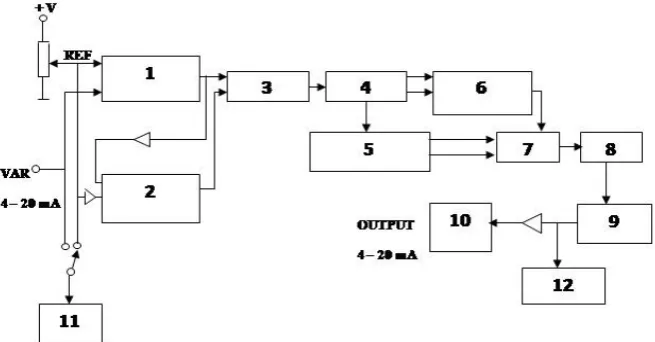
In Figure 1, the measured variable signal enters the

arithmetic circuit block (1), where it is multiplied with the value of the reference. The result of this operation has two paths: one of the entrances of the differential amplifier block (3) and one of the entrances of the arithmetic (2) circuit.

The result of the arithmetic circuit (2), is multiplied with the reference value and the result is applied to one of the entrances of the differential amplifier block (3). Arithmetic circuit 1 is identical to the arithmetic circuit (2), being the arithmetic circuit 1 one of the operators of the second circuit. The result of the mathematical operation of the first and second circuits is the electronic equivalent of two continuous mathematical iteration steps. The difference between the results of these two mathematical steps is what determines what to do to develop the control signal, if the value of the controlled variable of the process is that less than the desired value or reference, the mathematical result of the first arithmetic circuit shall be less than the mathematical result of the second arithmetic circuit and vice versa.

The signal at the output of the differential amplifier (3), is the subtraction of the mathematical results of arithmetic circuits (1) and (2), and is a direct voltage signal of +/ - 5 volts at 0 Volts or 5 volts when the variable X reaches the value of the reference. This asymmetric signal goes directly to an asymmetric rectifier block (4) and according to the voltage level of correction the frequency of oscillation in the block is increased or decreased (6), while the signal in the detector block (5) allows us to know if the value of the variable is above or below the reference value. Signals detector (5) and (6) voltage controlled oscillator block pass to the electronic key (7) block, this block of digital counters (8) delivers its signal to an a/d converter block (9), the signal obtained in these amplified and it is the output signal from control in the block (10). The block (11) is to work in manual or automatic and the block (12) is the digital display of the team that allows the reading of the reference value, the value of the variable and output for the final control element.

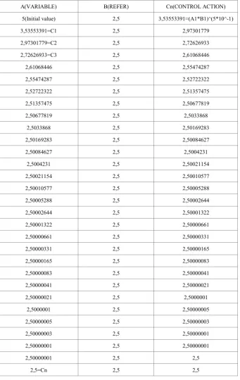
[image:2.595.141.469.531.702.2]

[image:3.595.136.478.89.630.2]

Table 1. Excel simulation

A(VARIABLE) B(REFER) Cn(CONTROL ACTION) 5(Initial value) 2,5 3,53553391=(A1*B1)^(5*10^-1) 3,53553391=C1 2,5 2,97301779

2,97301779=C2 2,5 2,72626933 2,72626933=C3 2,5 2,61068446 2,61068446 2,5 2,55474287 2,55474287 2,5 2,52722322 2,52722322 2,5 2,51357475 2,51357475 2,5 2,50677819 2,50677819 2,5 2,5033868

2,5033868 2,5 2,50169283 2,50169283 2,5 2,50084627 2,50084627 2,5 2,5004231

2,5004231 2,5 2,50021154 2,50021154 2,5 2,50010577 2,50010577 2,5 2,50005288 2,50005288 2,5 2,50002644 2,50002644 2,5 2,50001322 2,50001322 2,5 2,50000661 2,50000661 2,5 2,50000331 2,50000331 2,5 2,50000165 2,50000165 2,5 2,50000083 2,50000083 2,5 2,50000041 2,50000041 2,5 2,50000021 2,50000021 2,5 2,5000001

2,5000001 2,5 2,50000005 2,50000005 2,5 2,50000003 2,50000003 2,5 2,50000001 2,50000001 2,5 2,50000001

2,50000001 2,5 2,5

[image:4.595.60.294.78.462.2]

Figure 2. The variable star in value 5

Figure 3. The variable star in value 1

The Table 1 is the equations simulation using Excel program. If the Reference value is equal to 2,5 and the initial value of the Variable is equal to 5, in the iterative process the variable go to 2,5 value. With the same value of the Reference, but now the Variable starting in value equal to 1, in the iterative process the variable go to 2,5 again.

3. Functions Decomposition Method for

Finite Difference (DFDF) as a Tool to

Determine the Behavior of Functions

The DFDF method is a mathematical tool created with the aim of making a particular function into one that allows us to get more information about the original function as information obtained directly from it.

Generally applying n times the DDF method to a given function leads to properties of the function in question. For example, the factorial function xn exponent n by applying the method as many times as the exponent value is obtained. In other cases it leads to a periodic function as when the method is applied to log10 x-1 function, or to function as a constant value when applied to convert degrees to radians, ect.

The FDD method can be applied to any function and the analysis result can draw important conclusions that allow us to give other applications already known functions, or study the characteristics of unknown functions.

Definition

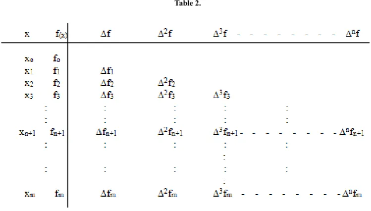
[image:4.595.62.294.79.252.2]

Let the function f (x) any function in which give to the variable x consecutive numerical values and whole, to make a discretized table with equidistant arguments (xi = x (i-1) + h,

1

≤ ≤

i m

, with h constant table showing the passage of the table) and their differences to the nth (

n m

≤

):

[image:4.595.115.490.507.720.2]

Table 1 is the 1st finite difference rearward of the function f at the point (xi, fi∆), defined as

∆fi=f(xi)-f(xi-1) (1) If g is denoted by the discrete function obtained, g (xi) =

∆f(xi), then the first backward finite difference g in xi is given by:

∆gi = g (xi) - g (xi-1) = ∆f (xi) - ∆f (xi-1) = [f(xi) - f(xi-1)] - [f(xi-1) - f(xi-2) ]

= fi - 2fi-1 + fi- (2) allowing 2nd define finite difference back of f at the point (xi ,

∆fi )in terms of the first:

∆2_f

i = ∆(∆fi) = ∆fi - ∆fi-1 (3) In general, the n-th finite difference of f at the point xi can be expressed recurrently in terms of finite difference of order n -1:

∆n_f

i = ∆(∆n-1fi) = ∆n-1fi - ∆n-1fi-1 (4) This expression is that calculates columns of the table. The expression (1) literally means that we make the subtraction between the current value and the previous one, and set the result at the level of the current value.

Needless to say, the construction is not mandatory for all columns to the nth finite difference. The number of columns we get to analyze depends on what we know we are studying specific function and perhaps with a ready-made column only get what we wanted. Hence, the method is very flexible and gives us the opportunity to develop our own creativity in

what we are investigating.

When we have a specific function and analyze the information provided to us is what we see directly and does not allow us to establish any relationship that may exist with numerical values given to the variables in question. For example, the function fixj = x2 tells us that the result is equal to a value x multiplied by itself; but it tells us the relationship that may exist between different numerical values given to the variable x. For this reason it was thought that the DFDF method.

We return to the analysis of the method definition. Consider the general expression (4) for n = 3,

∆3_f

i = ∆(∆2fi) = ∆2fi - ∆2fi (5) But considering (2) and (3)

∆3_{f = (f}

i - 2fi-1 + fi-2) - (fi-1 - 2fi-2 - fi-3)

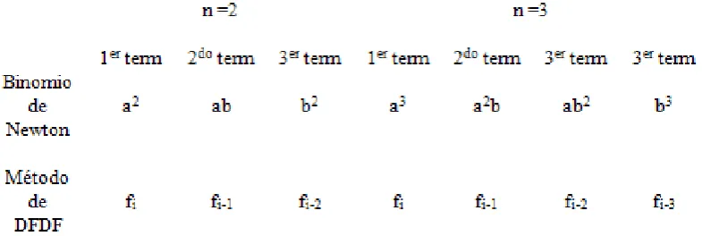
= fi - 3fi-1 + 3fi-2 - fi-3 (6) Note that the coefficients (2) and (6) are equal to those of Newton's binomial formula [5][6] (a - b) n _{for n = 2 and 3} respectively:

(a -b)2 _{= a}2_{- 2ab + b}2 (a -b)3 _{= a}3_{- 3a}2_{b +3ab}2 _{- b}3

[image:5.595.112.505.490.622.2]

But only coefficients are equal, as in Newton's binomial theorem we have two values are a and b, and these values are the product of them and those accompanying such coefficients, while the method will dfdf n + 1 values of the function accompanying coefficients, ie n + 1 are the above values that has taken the function analyzed.

Table 3.

[image:6.595.111.497.76.222.2]

Table 4.

In the first decomposition (

∆

X

m

=

X

m2

−

x

m2−₁) we saw that the difference between the values obtained was constant and this is what determines a second decomposition is made (

∆

2

X

_m−1

=

∆

X

_m

−

∆

X

_m−1), and of general conclusion we can say that for n = 2, the function f (x) = x2 _{for successive values of x to decompose twice obtain a constant value. If we do the} reverse process, that is, we go back and forth horizontally, we can obtain an equation that will give us the relationship between the values taken by the function f (x) = x2 _{for successive values of x; we effect taking the equations lead the columns:}

K

X

X

X

m

=

∆

m

−

∆

m

=

∆

2 _{−1 −1 (7)} 2

1 2

−

∆

−

∆

=

∆

X

_m

X

_m

X

_m (8) 2

2 2

1

1 − −

−

=

−

∆

X

_m

X

_m

X

_m (9) Substituting (8) and (9) in (7) and rearranging:

K

X

X

X

m2

−

2

m2−1

+

m2−2

=

(10) Take three consecutive decimal places and substitute in the expression (10):

(0.03)2_-2(0.02)2_+(0.01)2_=K 0.02=K

K=2(10-2₎

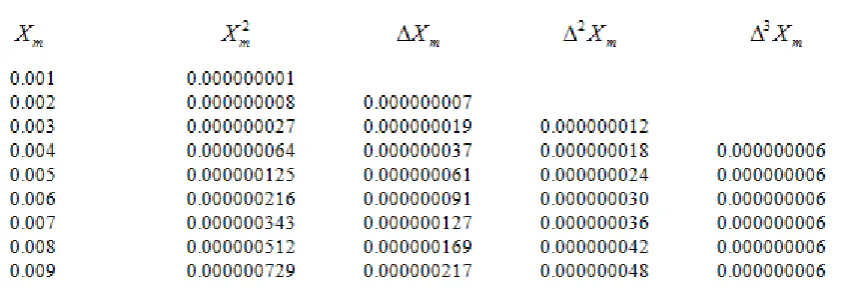
To get a general idea to do the same with the function f (x) = x3_{, taking the values 0.001, 0.002, 0.003, ..., 0.009;} decomposition and apply as many times as necessary to obtain a constant value.

Table 5.

[image:6.595.96.525.530.674.2]

[image:7.595.119.297.420.567.2]

Table 6.

Now the value of K = 6. When values are decimal thirteenth consecutive K value is multiplied by 10 raised to an exponent equal to the number of decimal places the value of the exponent of the function and negative.

If for x2_{, K = 2 and x}3_{, K = 6 can conclude that for xn, K =}

!n, that is, the constant K is equal to the factorial of the exponent of the function if the values of xm are integers. If these values are decimal:

K=n!(10-d_{) (11)} where: d = (No _{of decimal places) with exponent function}

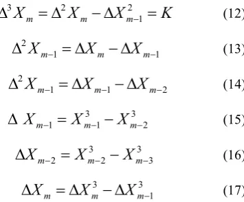
For this case:

K

X

X

X

m

=

∆

m

−

∆

m

=

∆

2₋

1 2

3 ₍₁₂₎

1 1

2

− −

=

∆

−

∆

∆

X

_m

X

_m

X

_m (13)

2 1 1 2 − − −

=

∆

−

∆

∆

X

_m

X

_m

X

_m (14) 3

2 3

1

1 − −

−

=

−

∆

X

_m

X

_m

X

_m (15) 3

3 3

2

2 − −

−

=

−

∆

X

_m

X

_m

X

_m (16) 3 1 3 −

∆

−

∆

=

∆

X

_m

X

_m

X

_m (17) Substituting (15) and (16) (14); (15) and (17) (13) and the results of (13) and (14) (12), we obtain by regrouping terms:

x_m3 x_m x_m x_m d 1 3 2 3 3 3

3 3 3 10

− ₋ + ₋ − ₋ = ⋅ −

( ) ( ) ( ) ! (18) Doing the same process for f (x) = x4 and f (x) = x5, we have:

xm4−4x( )4m−1 +6x(4m−2)−4x(4m−3)+x(4m−4)= ⋅4 10! −d (19)

xm5−5x(5m−1)+10x(5m−2)−10x(5m−3)+5x(5m−4)−x(5m−5)= ⋅5 10! −d (20) Taking the equations (10), (18), (19) and (20) we see that with them we can form the Triangle of Pascal [5][6] for binomial coefficients Newton. For X1 _{is obvious that the} equation is:

x

m

−

x

(m−1)

=

1

!

(21) For xo _{is :}

x

mo

=

1

x0 ₁

x1 _{1 1}

x2 _{1 2 1}

x3 _{1 3 3 1}

x4 _{1 4 6 4 1}

x5 _{1 5 10 10 5 1}

In this way we can obtain the coefficients for any order n; the signs are easy to allocate because alternating greater and the sign of the value of x is always positive and is also the first. The result of the equation is a constant and equal to the factorial of the exponent function. If x is less than zero value, then the result is n! (10-d), where d = (No _{of decimal places)} n. The decomposition has to be done as many times as the exponent and the equation has (n + 1) terms, that is, that (n + 1) are related consecutive numbers to always give a constant. Note the amount of information we have obtained by applying the method to the twelfth DFDF function and you do not even have imagined existed and could also obtain a general expression for the numerical value of an unknown term (m + 1):

xn(m+1) = ⋅n!10−d +nxmn −bx(nm−1)+cx(nm−2)−...±x(nm n− ) (23) Furthermore, consider the abscissa xi of Table 1 expressed exponentially with base 10, that is:

x

i

= ∞ ⋅

10

d (24)

where αand d are integers. As x are equidistant, then:

x

i−1

=

x h

i

− = ∞ −

(

1 10

)

d (25)

x

i+1

=

x h

i

+ = ∞ +

(

1 10

)

d (26)

from which it follows that the passage of the table is:

h

₌

₁₀

d

The function f (x) = xn _{has the following derivatives:}

f x

/

_{( )}

₌

nx

n−1 ₍₂₈₎

f x

//

_{( )}

₌

n n

₍

₋

₁

₎

x

n−2

(29)

f

///

_{( )}

x

₌

n n

₍

₋

₁

₎₍

n

₋

₂

₎

x

n−3 ₍₃₀₎

f

( )n

_{( )}

x

₌

n n

₍

₋

₁

₎₍

n

₋

₂

_)...(

n n

₋

₍

₋

₁

₎₎

x

n n−

₌

n

_!

(31) Finite differences can be seen, and in fact are approximations of derivatives, so we have:

h h x x h h x f x f h f x

f m m m mn m n

m) ( ) ( ) ( )

( / − − = − − = ∆ ≈ (32) d n d n d 10 ) 10 ) 1 (( ) 10 (∞⋅ − ∞− = d n n n d 10 ) ) 1 ( ( ) 10 ( ∞ − ∞− =

=

₁₀

(n−1)d

₍

∞ − ∞ −

n

₍

₁

_{) )}

n ₍₃₁₎

f

x

f

h

f x

f x

f x

h

m m m m m

//

_{( )}

_≈

∆

2

₌

( )

−

(

−

)

+

(

−

)

2 2 1 2

2

(34)

=

x

−

x

−

+

x

−

h

mn

2

mn 1 mn 2 2

=

(

∞ ⋅

10

)

−

2

((

∞ −

1

) )

+ ∞ −

((

2 10

)

)

10

2

d n d n d n

d

=

(

10

) [

∞ − ∞ −

2

(

1

)

+ ∞ −

(

2

) ]

10

2

d n n n n

d

=

₁₀

(n−2)d

_[

∞ − ∞ −

n

₂

₍

₁

₎

n

+ ∞ −

₍

₂

_{) ]}

n ₍₃₅₎

From (32) and (33) we can generalize:

f

x

f

h

n

n

n m

n m

h n d n n n n n nn n n

( )

_{( )}

_≈

₌

( −)

_[

_{∞ −}

_{( )(}

_{∞ −}

_{) ( )(}

₊

_{∞ −}

_{) .... ( )(}

_{− ±}

_{∞ − −}

₍

_{)) (}

_{± ∞ −}

_{) ]}

−

∆

10

2

1

2

1

1 2 1 (36)

Substituting in (29):

n

n n n n n n

n

n

n n n

!

≈ ∞ −

( )(

1

∞ −

1

)

+

( )(

2

∞ −

2

) ... ( )(

− ±

−1

∞ − +

1

)

± ∞ −

(

)

₍₃₇₎

Given (25), you are finally obtained:

x

mn

≈

n h

!

n

+

( )

1n

x

mn−1

−

( )

n2

x

mn−2

+

...

±

x

m nn− (38) proving the expression (23).

Example 1: Let

f x

( )

=

x

3_with

_x

o

=

0 001

.

and h=103, obtain the first three rows of the DFDF.

m xm f(xm)=x3 ∆fm ∆2fm ∆3fm 0 0.001 10-9

1 0.002 8*10-9 _7*10-9

2 0.003 27*10-9 _19*10-9 _12*10-9 (3 0.004 64*10-9 _37*10-9 _18*10-9 _6*10-9 ₎ and applying (36) and calculate

x

₃3 y

x

₄3:

3 3 1 3 2 3 3 3

3 3!(10 ) 3x 3x x

x ≈ ⋅ − + − +

≈ ⋅

_{6 10}

−9

+ ⋅

_{3 27 10}

⋅

−9

− ⋅ ⋅

_{3 8 10}

−9

≈

_{10 6 81 24 1}

−9

₍

+

−

+

₎

≈

_{64 10}

⋅

−9_,

x

43

≈ ⋅

3 10

!

−9

+

3

x

33

−

3

x

23

+

x

13

≈ ⋅

_{3 10}

_!

−9

+ ⋅

_{3 64 10}

⋅

−9

− ⋅

_{3 27 10}

⋅

−9

+ ⋅

_{8 10}

−9

With this we have achieved that knowing the previous four consecutive values of the function f (xm), we can determine the value to take the fifth value of this function without knowing the value of x5_{. So, we know the value it} will take in the future without the event has not yet occurred.

Example 2:

f x

( )

=

x

3con

x

_o

=

1

y

h

= ⋅

5 10

0 M xm f(xm)=x3 ∆fm ∆2fm ∆3fm

0 1 1

1 6 216 215

2 11 1331 1115 900

(3 16 4096 2765 1650 750 ) Checking using (36):

x

₃3 0 3

x

x

x

23 13 03

3 5 10

3

3

≈

!(

⋅

)

+

−

+

≈ ⋅

6 125 3 1331 3 216 1

+ ⋅

− ⋅

+

≈

4096

Applying again (36) calculate:

x

₄3

_{≈ ⋅}

_{3 125 3 4096 3 1331 126}

_!

_{+ ⋅}

_{− ⋅}

₊

≈

750 8295 126

+

+

≈

9261

The difference between Example 1 and 2 is that each x values are decimal and the two values are integers, putting forth what I said in the expression (11).

3. Conclusions

The research to find a mathematical equation to simplify the design and construction of industrial process controllers guided us to obtain:

1) An equipment with the following technical features: 4mA to 20mA input or 1volt 5 volt signal

Signal output of 4mA to 20mA or 1volt 5 volt input impedance: 250 ohms.

Output impedance: 100 ohm at 1000 ohms.

Digital indication in percent of the value of the variable and the value of the reference

Digital indication in percent of the value of the sign to the final control element Maximum time of compensation for delay of the final element of control and impulse lines: 60 sec

Maximum compensation of the speed of the process time: 240 sec

Possibility of working in mode of direct or inverse action

Mathematical parameters compensation for

temperature variations Consumption of 350mW

Power: 105 VAC to 130 VAC. Possibility of working with sensors active or passive.

2) It was possible to create a method of decomposition of functions by finite differences (DFDF) which also allows the analysis of functions is able to generate mathematical limits for these functions and establish a mathematical relationship between the process and the driver that leads to a new theory in the field of automatic control.

DFDF method is a mathematical tool created in order to make a certain function that allows us to obtain more information of the original feature that information obtained directly from it. In general the application of n times of the DFDF method to a given function leads to properties of the function in question. For example, the function Xn gets the factorial of the exponent n to apply the method as many times as the value of the exponent. In other cases, it leads us to a periodic function as when the method is applied to the l function log10 x-1, or a function of constant value as when applied to the conversion of degrees to radians, ect.

3) The design of a virtual machine similar to using LabView that much cheaper production costs and allows the use of large numbers of virtual drivers as control loops exist in the same industrial area using only a computer.

REFERENCES

[1] O´Dwyer; A Summary of PI and PID Controller Tuning

Rules for Process with Time Delay. Part 1: PID Controller Tuning Rules, Worshop on Digital Control: Past Present and Future of PID Control, Terrasa, España, Abril 5-7,2000

[2] O´Dwyer; A Summary of PI and PID Controller Tuning

Rules for Process with Time Delay. Part 2: PID Controller Tuning Rules, Worshop on Digital Control: Past Present and Future of PID Control, Terrasa, España, Abril 5-7,2000

[3] Shinskey, FG: Process Control Systems, Segunda Edición, Mew York, NY, EUA, McGraw-Hill Book Co.,1979

[4] Miranda Díaz L.J., Invention Patent Certificate, CU 23143 , Regulador Aritmético Radical Electrónico Para La Automatización De Procesos Industriales 2006.04.14

[5] Bernard Kolman & David R. Hill Algebra Lineal, 8va Edición