Maximum length sequence and Bessel
diffusers using active technologies
Cox, TJ, Avis, MR and Xiao, L
http://dx.doi.org/10.1016/j.jsv.2005.02.019
Title
Maximum length sequence and Bessel diffusers using active technologies
Authors
Cox, TJ, Avis, MR and Xiao, L
Type
Article
URL
This version is available at: http://usir.salford.ac.uk/428/
Published Date
2006
USIR is a digital collection of the research output of the University of Salford. Where copyright
permits, full text material held in the repository is made freely available online and can be read,
downloaded and copied for noncommercial private study or research purposes. Please check the
manuscript for any further copyright restrictions.
Final revised version 1
Maximum length sequence and Bessel diffusers using active technologies
Trevor J. Coxa,* , Mark R Avisa, Lejun Xiaob
a
Acoustics Research Centre, University of Salford, Salford M5 4WT, UK
b
Dept. of Electronic, Electrical & Computer Engineering, University of Birmingham, Birmingham, B15 2TT, UK
Abstract
Active technologies can enable room acoustic diffusers to operate over a wider bandwidth than passive devices, by extending the bass response. Active impedance control can be used to generate surface impedance distributions which cause wavefront dispersion, as opposed to the more normal absorptive or pressure-cancelling target functions. This paper details the development of two new types of active diffusers which are difficult, if not impossible, to make as passive wide-band structures. The first type is a maximum length sequence diffuser where the well depths are designed to be frequency dependent to avoid the critical frequencies present in the passive device, and so achieve performance over a finite-bandwidth. The second is a Bessel diffuser, which exploits concepts developed for transducer arrays to form a hybrid
absorber-diffuser. Details of the designs are given, and measurements of scattering and impedance used to show that the active diffusers are operating correctly over a bandwidth of about 100Hz to 1.1kHz. Boundary element method simulation is used to show how more application-realistic arrays of these devices would behave.
Keywords: Diffusers, Room Acoustics, Active Impedance, Bessel Arrays, Maximum Length Sequences
1. Introduction
Diffusers can be used to improve the acoustics of spaces [1]. This paper concerns studies of diffusers which incorporate active technologies. In a previous paper on active diffusers [2], it was demonstrated that active diffusers could provide wider bandwidth diffusion than passive devices. Adaptations of standard passive diffuser technologies were tested: the first device was a quadratic residue diffuser [3] with extended bandwidth, and the second a hybrid absorber-diffuser [4] which provided partial absorption while diffusing reflected sound. This paper concerns the use of active technologies to achieve finite bandwidth diffusers which are difficult to achieve passively; indeed, equivalent passive versions can only be made to work at single or discrete frequencies.
The first part of the paper looks at forming patches on the diffuser surface which have pressure reflection coefficients of minus one: i.e. areas where the phase of the pressure is inverted on reflection. As will be discussed below, it is possible to form such patches through passive means using a well which is a quarter of a wavelength deep, but the pressure inversion is only achieved for a set of discrete frequencies. Using active technologies, it is possible to produce pressure inversion for all frequencies over a bandwidth of several octaves; this is equivalent to employing a diffuser well whose depth varies with frequency. Consequently, it is possible to surpass the performance of a passive design by using this active equivalent of a Maximum Length Sequence (MLS) diffuser [5].
The second part of the paper looks at using Bessel array technologies [6]. Bessel functions are used in the determination of elemental source-strengths within loudspeaker arrays to enable a more spatially uniform radiation. As the mathematics behind Schroeder diffusers has much in common with transducer array design, a similar Bessel approach can be adapted for diffusers. The authors are unaware of previous attempts to construct Bessel diffusers using passive means, perhaps due to the aforementioned bandwidth limitations for
*
Corresponding author. Tel: +44 161 295 5474, Fax: +44 161 295 4442.
passive surfaces. Using active technologies, however, it is possible to develop a Bessel diffuser that operates over a three to four octave bandwidth. This part of the paper includes two novel designs, one passive and one active.
The paper begins by describing briefly the active control system used. It then describes the work on maximum length sequence diffusers, and finishes by examining the Bessel diffuser.
2. Overview
As the active control technologies used in this paper have been described in detail in reference [2], only a brief overview is given here. Fig. 1 shows a typical construction of the maximum length sequence diffuser tested in this paper. An active impedancesystem is used to achieve the desired impedance at the control surface. For instance, this impedance may be set such that the impedance at the well mouth is zero, which relates to a reflection coefficient R=-1. To achieve this, the control loudspeaker is instrumented to measure pressure and velocity, and from this the surface impedance calculated. This measured impedance is used in conjunction with an adaptive controller to drive the impedance towards a desired value. The work here mostly uses a feedforward topology, exploiting a control regime first developed for active absorption.
2.1. Maximum length sequence diffusers
Schroeder began his work on diffusers by investigating the scattering from maximum length sequences [5]. The MLS diffuser proposed by Schroeder is an ancestor to the active diffuser proposed here. Fig. 2 shows one period of a passive MLS diffuser based on a length 7 sequence: {0,0,1,0,1,1,1}. Schroeder chose to use maximum length sequences because they have a flat power spectrum at all frequencies (except dc). There is a close relationship between the reflection coefficient power spectrum and the surface scattering. Indeed, it is well established in optics that the far field scattering can be found from the Fourier Transform of the surface reflection coefficients; although for acoustic diffusers the applicability of this principle is more limited than in optics. While more complex prediction models, such as Boundary Element Methods (BEMs), can be used to gain more accurate results, the simpler Fourier-based model enables a better insight into the problem and the design principles. This will be referred to as the Fraunhofer model. The most simplified version of this prediction model states that pressure magnitude |p| is given by [7]:
s jkx dx e x R Ap
,
cos(
) ( ) [sin()sin()] (1)Where is the angle of receiver to the surface normal; the angle of incidence to the surface normal; A is a constant; R(x) is the surface pressure reflection coefficient; k the wavenumber, and x the distance along the surface. The prediction is being carried out in one plane only.
equal to half a wavelength, the surface behaves like a plane surface because R=1 for all parts of the surface; this is a critical or flat plate frequency. Consequently, the MLS diffuser is only useful over a limited bandwidth, which at most is an octave.
Using active technologies it should be possible to extend the bandwidth of the diffuser so that the desired reflection coefficient is achieved over a wider frequency range. The active element must effectively simulate a well whose depth varies with frequency.
2.1.1. Forming the desired impedance
The structure that was tested is shown in Fig. 1. The results presented here are for a single active controller in the central well; the final device requires multiple controllers in one spatial period. The active controller in the centre well has to generate a reflection coefficient of minus one at the well entrance. The control surface is mounted within a well since the one-dimensional environment greatly simplifies the control task – only plane wave propagation is considered.
It is necessary to calculate the required impedance at the control surface to achieve the desired impedance at the well entrance. A transfer function matrix method (also known as a two port model) can be used to relate the impedances in the wells. Fig. 4 shows the arrangement being considered. The impedance at the control surface, z1, is related to the termination impedance of the virtual well, zT, by [7]:
k d d
c j z c d d k jz c z T T ' cot ' cot 1
(2)To achieve an impedance at the well entrance of z2=0, equivalent to R=-1, the virtual well should be a quarter wavelength deep. Mathematically this can be expressed as kd’=(2n-1)/2, where n is an integer. When this is incorporated into Eq. (2), the control impedance becomes:
kd c j z c kd jz c z T T tan tan 1
(3)This implies that for a non-absorbing controlled termination where zT, the desired control impedance is –
jρc tan(kd). This desired termination impedance must be represented by a filter within the control system, which poses problems. An Infinite Impulse Response (IIR) filter based on a transfer function z1 = -jρc tan(kd) is unstable, and a Finite Impulse Response (FIR) filter structure is non-causal. The lack of stability can be overcome, however, by limiting the bandwidth over which the desired impedance is controlled.
While it might at first seem desirable to achieve very wideband control, in practice control is only required over a wide but reduced bandwidth. Tests on a variety of active diffusers [2] and absorbers [10] have shown that broadband stable and robust control can be achieved over about 3-4 octaves, say from 100Hz to 1kHz. Above 1kHz, it is difficult to design this type of active control system to behave in a stable manner, and errors in transduction become increasingly problematic. Furthermore, as the control impedance has a series of singularities at kd=(2n+1)π/2, n=0,1,2,... limiting the bandwidth of operation helps by placing these singularities above the frequency range of active control and so the singularities do not directly cause problems. Fortuitously, it is relatively easy to provide passive diffusion above 1kHz and so limiting the bandwidth is not a significant limitation. Consequently, the upper frequency limit comes from a combination of the limitations of the active control system, the desired termination impedance function and the frequency at which passive diffusion is easy to achieve.
Fig. 5 shows the broadband impedance required (which is unstable) and the stable, band-limited target filter function which achieves a match with the desired impedance over a more limited frequency range. This band-limited filter is an 8th order IIR type. The locations of the poles and zeros were found using a numerical optimization; the sum of the squared, complex differences between the target and achieved transfer functions were minimised over a finite bandwidth. The order of the filter and the lower frequency limit of the
optimization process (200Hz) were found by trial and error. It is possible to achieve a filter that matches the desired impedance to a rather lower frequency, provided that the order of the filter is increased to achieve a reasonable match across the whole desired bandwidth. Fig. 5 also shows the actual impedance measured at the controller. The controller is providing the required surface impedance from roughly 200Hz to
1kHz. When translated to the impedance at the well mouth using a transfer matrix calculation, it is found that the impedance is actually satisfactorily controlled from 100Hz to 1.1kHz. The bandwidth is wider, because the sensitivity of the well mouth impedance to errors in the control surface impedance varies with frequency, and in this case, between 100-200Hz and 1-1.1kHz the well mouth impedance is not that sensitive to control surface impedance errors.
Within the control structure, a Least Mean Square (LMS) [11] algorithm operates on the error between the actual and desired velocity to update the coefficients of an adaptive filter. The LMS algorithm reduces the error by changing the filter coefficients, to match as best as possible the desired and measured impedance at the control surface. It is necessary to prevent the LMS algorithm considering errors outside the operational bandwidth. To achieve this, the error signal was low-pass filtered using an 8th order IIR Butterworth filter, with a -3 dB point of 1.1kHz.
2.1.2. Scattering measurements
To confirm that the diffuser is performing as designed, a 2D test environment was used as outlined in reference [2]. The test environment measures the scattered polar response from the diffuser, which is the usual method for evaluation. A passive diffuser was constructed, as shown in Fig. 2, to be compared to the active diffuser. If the active diffuser works correctly, then the scattering from both surfaces should be identical at the design frequency where the wells of the passive diffuser are a quarter of a wavelength deep (500Hz).
Fig. 6 shows the scattering from the active diffuser, compared to a passive diffuser of greater overall depth. At the intended test frequency of 500Hz, the passive and active diffusers produce very similar scattering, demonstrating that the active well is behaving as intended. At 1000Hz, the passive diffuser suffers from a flat plate frequency where the well depth is half a wavelength, and consequently the waves reflecting from all parts of the surface are in phase. The passive diffuser therefore produces scattering like a plane surface. The active diffuser, on the other hand, does not suffer from this problem because the reflection coefficient for the central well is still minus one, and consequently, it is still producing scattering. These measurements
demonstrate the utility of the active diffuser in producing scattering over a broader bandwidth than a passive MLS diffuser and avoiding flat plate frequencies.
2.1.3. Simulation study
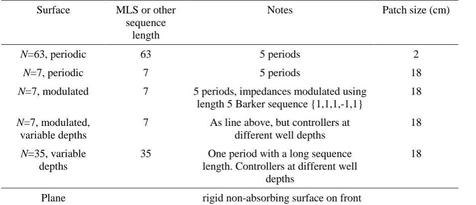
The prediction study used 5 periods of the diffuser, each period being 1.26 m wide. Various models were examined as summarized in Table 1. Two different lengths of MLS sequence were used, because patch size has an important effect on scattering quality. Modulated diffusers were also tested; this is described in the next section. For the active wells, the low frequency surface impedance (<1100Hz) was taken from the measurements on the active controller. Above 1100Hz, when the controller no longer works, the impedance was calculated assuming a stationary control surface presenting a rigid termination. The scattering was predicted in the far field at discrete frequencies. The results were converted into 1/3 octave bands by integrating the scattered energy from nine discrete frequencies within the 1/3 octave bandwidth using Simpson’s rule.
2.1.3.1. Modulation
Work on passive diffusers has shown that the period width is important, because this determines the angular location of any grating lobes. If only a few grating lobes are present, they form a dominant feature in a scattered pressure polar response, and can lead to uneven scattering. Consequently, methods have been developed which allow the period width to be increased, or indeed any repetition to be completely removed. Increasing the period width is also important, because otherwise the low frequency performance of a diffuser can be limited [7]. As a result, the issue of periodicity is very important to the design of active diffusers which are designed to operate at low frequencies.
Angus [13-14] presented a series of papers outlining methods to reduce repetition by using two quadratic residue diffuser base shapes in a modulation scheme. This process can also be applied to active diffusers. Fig. 7shows one of the modulation arrangements tested. As discussed previously, the far field scattering distribution is related to the Fourier Transformation of the surface reflection coefficients. For a periodic device, the distribution of reflection coefficients, R(x), can be expressed as the reflection coefficients over one period, convolved with a series of delta functions giving the location of each period of the device:
n nnW
x
x
R
x
R
(
)
1(
)
(4)where R1(x) is the distribution of reflection coefficients over one period; n is an integer;٭ denotes
convolution; W is the width of one period of the device, and is the delta function.
When a Fourier transform is applied to Eq. (4) to obtain the scattering in sin()+sin() space, then the convolution becomes multiplication:
n nnW
x
FT
x
R
FT
x
R
FT
(
)
1(
)
(5)Here, FT{} denotes Fourier Transform. The Fourier Transform of a delta function train is another delta function train, and it is the peaks in this second train for sin()+sin()>0 that cause the grating lobes. Consequently, rather than use a delta function train to form a periodic device, another function should be used which has better Fourier Transform properties. A modulation sequence with excellent autocorrelation properties is needed and a good choice is a Barker sequence. This is a binary sequence whose autocorrelation has the lowest possible sidebands [15]. Consequently, the response of the whole array of diffusers is closer to the single diffuser alone than if a periodic arrangement is used. If a perfect binary sequence could be found, then the single diffuser response would be recovered, but there is only one such 1D sequence (which has length four).
The Barker Sequence for N=5 is used as shown in Fig. 7, {1,1,1,-1,1}. Consequently, where a 1 appears in the Barker sequence, the normal diffuser should appear. Where a –1 appears, a diffuser which produces the same, but phase-inverted, scattering is used. This can be achieved by inverting the initial diffuser profile, and is equivalent to modifying the phase change due to the well depths from to 2-. To evaluate how
effective the modulation is, another diffuser with no repetition was formed from a single binary sequence of length 35 for comparison {1, 1, 1, 1, 1, 1, 1, -1, 1, 1, -1, -1, 1, -1, -1, 1, 1, -1, 1, -1, 1, -1, -1, 1, -1, 1, -1, 1, 1, 1, -1, -1, -1, 1, 1}. The sequence used was one which has been found to have the best aperiodic
2.1.3.2. Results
Fig. 8 demonstrates the usefulness of modulation in improving the low frequency performance of the active diffusers. At this frequency, 200Hz, only the zeroth order (specular) lobe is generated by the periodic surface, because the wavelength is greater than the period width. Consequently, the periodic structure is producing a reflection similar to a plane surface. The modulated diffuser shows additional dispersion because it is able to produce more obliquely propagating sound. At or below 200Hz, the device based on a single period of length 35, is better than the length 7 diffuser modulated using the Barker sequence. This might be because the length 5 Barker sequence has significant side bands in the autocorrelation function (it has a relatively low merit factor [15]), and consequently uneven scattering. Above 200Hz, there appears to be no advantage to using a longer sequence over a modulated one.
Fig. 9 also shows another case where increasing the repeat distance improves performance. This is a frequency (500Hz) where the wavelength is smaller than the repeat distance for the periodic device and so three grating lobes are generated. The length 35 device has no periodicity, and so the scattering is more even as periodicity lobes are not present. Above 800Hz, the effects of periodicity become less important. For the periodic device, the number of lobes becomes significantly large and the scattering becomes more even.
Results showing the usefulness of lengthening the repeat distance have been seen at higher frequencies for passive diffusers, but have not been examined at such low frequencies before. Due to the relative long wavelengths involved, the low frequency limit of diffusion is more likely to be determined by repeat distance for active diffusers. Consequently, particular care is needed to remove repetition.
Above 1100Hz, the active controller is ineffective and so the reflection coefficients are no longer determined by a maximum length sequence. The performance of the diffuser is now dependent on the appropriate arrangement of the active elements (now acting with approximately rigid termination) in association with the zero depth wells. A design where all the active elements are at the same depth will suffer from critical frequencies, and when the well depth is equal to half a wavelength the reflected wavefront will resemble that for a plane surface. Fig. 10 compares a plane surface with a diffuser with three active elements all at the same depth. This is close to a critical frequency (the critical frequency actually lies at the edge of the one-third octave band shown), and the scattering from the diffuser is poor. This problem is overcome by varying the depths of the active controllers. By choosing depths related by primes, say in the ratios: 2 : 3 : 5 : 7 large frequency. Moreover, this ensures that the frequencies at which the reflected waves from two or three of the wells are in phase, where there might be a lack of phase variation across the front of the diffuser, are also placed at as high a frequency as possible. Even better is to use a non-integer ratio between the depths to ensure there are no exact critical frequencies. This can be most easily done by using fractions of prime numbers. So depths were set according to ratios 1/2 : 1/3 : 1/5 : 1/7, where the deepest active well was 15 cm long. Fig. 10 shows the scattering from this design, and an improvement over the diffuser with equal active well depth can be seen.
Above 1100Hz, the quality of scattering is not particularly good, and better passive diffusers can be
designed. The design of the diffusers started by concentrating on the bandwidth over which active control is achieved, and only then were the higher frequencies considered. By considering both frequency ranges at the same time, say by using numerical optimisation [17], it might be better to further improve performance. The limited performance probably arises because about 50% of the diffuser surface consists of zero depth wells producing a coherent specular reflection, and while this effect can be modified by interference from the wells of variable depth, a large flat area at the front of the diffuser limits the performance achievable. This might be solved by bending the whole diffuser and so creating additional wavefront dispersal. A further problem is that at higher frequencies, the width of the wells is too wide compared to wavelength. Reducing the patch size can help, but then the low frequency performance is compromised. This has been previously shown with active hybrid absorber-diffusers [2], and similar trends were found for the active devices tested here.
2.2. Bessel Diffusers
2.2.1. Design
By changing the relative phase and magnitude of signals driving each transducer in a loudspeaker array, it is possible to change its directivity in order either to make it more omni-directional, to steer the main lobe in a particular direction, or to generate a focussed beam. Bessel transducer arrays use inter-element source strength relationships determined from Bessel functions. The resulting array radiates with a similar directional response to one element, but with increased power. This part of the study set out to investigate whether this concept could be adopted for diffuser design.
Bessel functions have the following mathematical property [6,18]:
constant
)
(
n jn nz
e
J
(6)Where Jn(z) is the Bessel function of order n; z and Ω are constants. This can be compared to the simple Fraunhofer prediction model for scattering from a diffuser, to reveal how this property might be exploited in diffuser design. The scattering from the diffuser represented by Eq. (1) can be simplified to a sum over the wells:
sin( )1 0
2
)
sin(
)
cos(
jknw N n ne
R
kw
sinc
w
A
p
(7)Where w is the well width; sinc(a) = sin(a)/a; n is the well number, and there are N wells in total. Normal incidence has been assumed. The reflection coefficients of the diffuser are set using Bessel functions, i.e. Rn = Jn(z)/s where s is a scaling constant. Eqs. (6) and (7) can then be combined if Ω is equated with kw sin(θ). Under these conditions, for a diffuser with a very large number of wells, it can be shown that the pressure magnitude scattered from the diffuser then reduces to:
2
)
sin(
)
cos(
w
sinc
kw
s
A
p
(8)Eq. (8) is identical to the scattering from a single zero depth well (consider Eq. (7) with N=1 and R0=1), except for the addition of the scaling constant s. This suggests that provided the reflection coefficients of the diffuser are set using Bessel functions, then the scattering from the whole diffuser will have the same polar distribution as from a single well alone (except for a simple scaling of the overall sound power reflected). Provided that the wells are narrow compared to wavelength, then the scattering from the single well should be relatively omni-directional, and so the whole diffuser array should produce relatively uniform scattering. This behaviour is directly analogous to the radiation properties of the Bessel transducer array described previously.
In theory it is necessary to have an infinite number of wells to exploit the property of Eq. (6), but it is possible to truncate the infinite sum without greatly changing the scattering. Fig. 11 shows the values of
Jn(z)/s for z=1.43and s=0.55for 21 values of n. As |n| increases, the value of Jn(z)→0, which implies that the outer wells should have reflection coefficients Rn→0. As these outer wells would not contribute greatly to
the scattered pressure, there is no need to include them in the diffuser, and so it is possible just to use a small number of wells when making the diffuser. In the case of Fig. 11, it is possible to construct a diffuser with just 7 wells.
chosen so that the maximum value of the reflection coefficient was 1, as this can be generated by a simple rigid termination.
A maximum of three active wells could be simultaneously implemented using the DSP board available for this study, and so it was necessary to identify a series of reflection coefficients which only required three actively controlled wells, with the remainder being formed by passive means. Fortunately, this could be achieved. The sequence of reflection coefficients Jn(z)/s shown in Fig. 11 is {-0.097, 0.39, -0.99, 1.00, 0.99, 0.39, 0.097}. The series can be approximately represented by the reflection coefficients {0, 0.39, -1.0, 1.0, 1.0, 0.39, 0} as shown by the squares in Fig. 11. Fig. 12 shows the resulting diffuser. The R=0 wells are shown filled with loosely packed mineral wool, offering characteristic impedance and hence complete absorption over the bandwidth of interest. For R=1 a non-absorbing zero-depth well was used. This left three active wells to be constructed. Tests using the simple Fraunhofer model showed that approximating the reflection coefficients as described here did not produce significant errors in the scattering from the array.
For the R=-1 well, the controller described previously for the MLS diffuser was used. For R=0.39, a new control regime was necessary. Initially, it was intended to control the impedance using a similar approach to the R=-1 case. For R=0.39, the normalised impedance at the well mouth needs to be z2=2.28. The control surface impedance is therefore found from a transfer matrix approach:
) cot( ) cot( 1 2 2 1 kd j z z kd j c z
(9)Within the DSP controller it is necessary to represent this desired controlled surface impedance, z1, as an IIR filter. Unfortunately, it proved impossible to fit this control impedance as the exact broadband transfer function represents an unstable filter. Even when band limited, a sufficiently-accurate digital approximation required a very high order filter, and in this case the impulse response has large transients which cause problems of dynamic range with velocity transduction at the control surface. The controller can also be configured to act using a desired admittance, but the reciprocal of Eq. (9) was equally difficult to implement. For this reason another approach employed, shown in Fig. 12. Thin woven metal mesh was obtained which offered a well defined resistance and negligible reactance. Fortunately, mesh having the desired surface resistance was available and could be used at the mouth of the well. With this resistance value already correct, the controller merely implements a pressure minimum behind the metal mesh to achieve the correct surface impedance.
To enable the experimental verification of the active diffuser, a passive equivalent was constructed which was designed to work at one spot frequency. This is also shown in Fig. 12. The R=-1 well was made by setting the depth to be a quarter of a wavelength. The R=0.39 wells were made by mounting a piece of mineral wool over an air gap. A process of trial and error was used to find the appropriate air gap and mineral wool with a sufficiently high resistance. This trial and error process was undertaken in an impedance tube. This passive equivalent was compared to the active diffuser in the 2D measurement apparatus.
2.2.2. Measurement results
2.2.3. Simulation study
Section 2.1.3 detailed the simulation study used for the MLS diffuser, and a similar philosophy is followed here. Table 2 shows the diffusers tested. The first diffuser is a periodic arrangement of the measured surface shown in Fig. 12. Up to a frequency of 1.1kHz the control surfaces are modelled as those produced by the active controller, above 1.1kHz, the control surfaces are modelled as rigid (to a first approximation). A transfer matrix calculation is undertaken to calculate the resulting impedance at the well entrance. It is anticipated that the periodic Bessel diffuser will suffer from grating lobes, and consequently modulation is used to remove periodicity and improve the scattering. In this case, the Bessel diffuser R = {0, 0.39, -1.0, 1.0, 1.0, 0.39, 0} is modulated with its inverse, i.e. a surface with R = {0, -0.39, 1.0, -1.0, -1.0, -0.39, 0}. The modulation sequence used is a Barker sequence based on N=5, as previously used and shown in Fig. 7. The inverse diffuser simulated is shown in Fig. 14. The R=-0.39 well is formed by placing a controller behind a wire mesh. Without the added resistance of the wire mesh, the required control surface impedance cannot be implemented as the digital filter is unstable - as was the case for R=0.39. In this case, it is not possible to simply minimize the pressure behind the wire mesh, since the desired reflection coefficient is negative, and the required controlled impedance must be calculated using a transfer matrix model.
A third Bessel diffuser was tested with a large number of wells (N=35) and no repetition. The reflection coefficients are calculated using Rn= Jn(z)/s, with z=14and s=0.286for -17 ≤ n ≤ 17; the values of z and s are again found by trial and error. The reflection coefficients of the well openings are shown in Fig. 15. This represents the ideal Bessel diffuser for covering a wide area because it will have no grating lobes because it has no repetition. However, the design does not form a very practical Bessel diffuser, since virtually every well would require active control to achieve the desired reflection coefficient, and it is likely that some of these reflection coefficients imply unstable control filters. However, it is useful to examine the scattering from this surface, because it gives a rough upper limit on the quality of scattering that might be possible from an ‘ideal’ Bessel diffuser.
2.2.3.1. Results
First the ‘ideal’ Bessel diffuser with no repetition (N=35) is considered; this device might be expected to exhibit optimum performance. Fig. 16a shows scattering for a frequency at which this diffuser functions exactly as expected. The plot compares the scattering from the Bessel diffuser predicted using a BEM model, with that predicted by Eq. (8). This confirms that Bessel sequences can be used to recover the scattering from a single well of the diffuser; the concept has been shown to translate from loudspeaker arrays to diffusers. However, the scattered energy tails off at grazing angles because of the cos(θ) factor shown in Eq. (8); the scattering from this surface mimics a Lambert’s cosine law distribution, rather than even scattering in all directions. (These results also demonstrate the utility of using a simple prediction models to understand simple trends in diffuser behaviour.) The lack of lobes in the scattered polar response is unusual for such a complex surface.
At lower frequencies the scattering from the N=35 Bessel diffuser is more uneven as shown in Fig. 16b. It is suggested that this happens because when the wavelength becomes large compared to the well width, the mutual interactions between the wells cause a significant alteration in the pressure distribution, and so the Bessel diffuser no longer behaves as intended. A further possible factor, is that the edge conditions of the diffuser become more important at low frequencies, and strictly speaking the Bessel diffuser should be mounted in an absorbent baffle.
At higher frequencies, the reflections are less well scattered, as illustrated in Fig. 17. In this case, the well width becomes significant compared to wavelength, preventing the diffuser behaving like the ‘ideal’ Bessel diffuser. The solution to this problem might be to use a fractal design, so that diffusers at different scales are used to scatter sounds at different wavelengths. It is unclear, however, how such designs might be
constructed using Bessel functions.
the modulated surface generates better scattering; for example, Fig. 18 shows the scattering from the periodic and modulated arrangements at 315Hz. At this frequency, the periodic device generates two side lobes due to spatial aliasing. The modulated device produces more even scattering; however, the modulation technique is not as successful as has been noted for some other designs, such as quadratic residue diffusers [7]. This might be because the Barker sequence used for this modulation is the length 5 sequence, which has a relatively low merit factor. From 800Hz upwards, there is little difference in the performance of the periodic and modulated diffusers. At 1kHz the scattering is most even, and this is illustrated in Fig. 19. Above 1.1kHz, the surface reflection coefficients deviate from their Bessel function target values, as the active controller cease to work. As frequency increases, the scattering gets less even. For high frequencies (see periodic device result in Fig. 17) the dispersion is actually worse than for a flat plane surface. This problem arises not only because the reflection coefficients are no longer ideal, but also because the well width becomes too large compared to wavelength as noted previously for the N=35 device.
2.3. Absorption of active diffusers
The absorption of a diffuser can be estimated from the BEM predictions. The scattered intensity for the diffuser is summed over the polar response and denoted, Id. The scattered intensity for a plane non-absorbing surface of the same size is summed over the polar response and denoted, Ip. Then the absorption coefficient,
, is estimated to be:
p d p
I
I
I
(10)The source and receivers in the BEM simulations were in the far field, meaning that the intensity could be simply related to the square of sound pressure.
Fig. 20 illustrates absorption coefficient for the Bessel and MLS diffusers. The absorption coefficients can be explained if it is assumed that there is intercell cancellation from the wells with opposite reflection
coefficient, similar to the cancellation which occurs for acoustic radiation from a vibrating, finite plate [19]. The reflection coefficients for the Bessel diffuser were shown in Table 2. If it is assumed that the radiation from the neighbouring R=-1 and R=1 wells cancel, then the absorption coefficient can be simply estimated from the surface reflection coefficients to be about 0.81, a value that approximates well in practice. At higher frequencies, this intercell cancellation no longer occurs; firstly, the well spacing becomes significant
compared to wavelength and secondly, the controlled reflection coefficient is no longer R=-1. For these reasons, the absorption coefficient drops to around 0.5. A similar model can explain the absorption coefficient of the MLS diffuser at 1kHz and below. Above 1kHz, the MLS diffuser absorption coefficient tends to zero; this is expected when intercell cancellation becomes insignificant, as the absorption of the surface itself is then minimal.
2.4. Discussions
The active MLS diffuser offers a method for achieving good diffusion in the bandwidth of operation of the control filters, but the performance needs to be improved at higher frequency. Due to intercell cancellation, the diffuser produces some absorption. For this reason, there will be applications for which this type of diffuser would not be ideal: for example in large concert halls for classical music where the preservation of acoustic energy is a paramount concern. In other spaces, such as studios, the loss of energy would not be so important.
for diffuser design and derived from number theory, the Bessel coefficients are not meant to be used in a periodic manner. A second, and more serious problem, is that scattering becomes poor at high frequency when the wavelength becomes small compared to the well width, and additionally the active controllers cease to generate the correct reflection coefficients at the well entrances. As with the maximum length sequence diffuser, it is suggested that some form of fractal construction [21] might help overcome the well width problem, but methods for developing a fractal Bessel diffuser are not as obvious as they are for Schroeder diffusers. This could also help overcome the problem of the reduction in scattering at higher frequencies when the active controllers stop working. Finally, the absorption coefficient of the Bessel diffuser is probably too high for a hybrid absorber-diffuser. A set of reflection coefficients with less intercell cancellation is needed so that more reflected sound is generated.
In a previous paper on active diffusers [2], an active hybrid diffuser was developed and tested where the impedance discontinuities between reflective and completely absorbing patches were used to create dispersion. These binary amplitude diffusers cause partial absorption, with the intention that any reflected energy is diffused, and so has similarities to the Bessel diffuser above. Fig. 21 compares the scattering from a Bessel diffuser and the binary amplitude diffuser at 1kHz. For 100Hz to 1kHz, the Bessel diffuser produces more even scattering that the binary amplitude diffuser. This is because the binary amplitude diffuser has a flat and reflective surface covering 50% of its area, meaning that the specular reflection can only be attenuated by 6dB at the most. Above 1kHz, the performance of the Bessel and binary amplitude diffusers are similar, although in both cases the dispersion is not great; a high frequency case for two Bessel diffusers was shown in Fig. 17. Consequently, the Bessel function offers better performance overall. However, the active binary amplitude diffuser can use a more simple feedback controller [2].
3. Conclusions
This paper has presented two new designs for active diffusers, one based on a maximum length sequence, the other on Bessel functions. While a maximum length sequence diffuser can be constructed passively, such designs only operate at discrete frequencies, and so their application is limited. The active maximum length sequence diffuser improves on the passive equivalent by simulating well depths which are frequency dependent, and so diffusion is created over a significant bandwidth. New passive and active diffusers based on Bessel transducer arrays were presented. The passive equivalent is very limited in that it only works at one frequency; this problem can be overcome by using actively controlled elements in the diffuser.
Measurements of scattering and impedance have shown the active diffusers work from 100Hz to 1.1kHz. Above this frequency range the active controllers no longer operate correctly. Boundary element method simulations have explored how these diffusers might behave when arranged in arrays. The simulations have confirmed the good performance of the diffusers over a reasonably wide bandwidth, but have shown weaknesses in their performance that indicate avenues for further research. There are also challenges regarding the use of multiple controllers that require further work before the large simulated diffusers can become reality, in particular overcoming the computation burden of adaptation when there are multiple controllers.
4. Acknowledgements
Table 1.
Models tested in BEM study for the maximum length sequence diffuser. All were 6.3m wide, 5cm deep, with the sides and rear modelled as being absorbent.
Surface MLS or other sequence
length
Notes Patch size (cm)
N=63, periodic 63 5 periods 2
N=7, periodic 7 5 periods 18
N=7, modulated 7 5 periods, impedances modulated using length 5 Barker sequence {1,1,1,-1,1}
18
N=7, modulated, variable depths
7 As line above, but controllers at different well depths
18
N=35, variable depths
35 One period with a long sequence length. Controllers at different well
depths
18
Table 2.
Models tested in BEM study for the Bessel Diffuser. All were 6.3m wide, 5cm deep, with the sides and rear modelled as being absorbent.
Surface Notes
N=7 periodic Bessel 5 periods, 7 wells per period, simulation of periodic arrangement of implemented active diffuser
(shown in Fig. 12)
R = {0, 0.39, -1.0, 1.0, 1.0, 0.39, 0}
N=7 modulated Bessel 5 periods, 7 wells per period, of implemented active diffuser modulated with its inverse.
(see Fig. 14 for inverse diffuser)
Figure Captions
Fig. 1. A cross-section through one period of an active maximum length sequence diffuser. Only the middle active element is shown instrumented. Dimensions in cm.
Fig. 2. A cross-section through one period of an N=7 maximum length sequence diffuser.
Fig. 3. The scattering from 5 periods of an N=7 MLS sequence at its design frequency. MLS diffuser
plane surface
Fig. 4. Geometry for calculating well impedance. d’ is the length of the virtual well, which in this case is frequency dependent. z1, z2 and zT are the impedances at the positions shown on the diagram.
Fig. 5. Filter functions to achieve a pressure reflection coefficient of -1 at the well entrance: the desired broadband impedance function jpc tan(kd);
the target impedance, a stable filter function over a limited bandwidth, and the achieved impedance as measured with the active controller in operation.
Fig. 6. The scattering from three surfaces at two different frequencies. Plane surface;
Active MLS diffuser; Passive MLS diffuser.
Fig. 7. Modulation scheme for the active diffusers. The number sequence at the bottom indicates the modulation sequence used, and the change in shading is used to emphasise the inverted diffuser.
Fig. 8. Scattering from three surfaces for 200Hz 1/3 octave band. Plane surface;
N=7, periodic;
N=7, modulated.
Fig. 9. Scattering from three surfaces for 500Hz 1/3 octave band. Plane surface;
N=7, periodic;
N=35.
Fig. 10. Scattering from three surfaces for 2kHz 1/3 octave band. Plane surface;
N=7, modulated, active controllers all at the same depth;
N=7, modulated, active controllers at different depths.
Fig. 11. Scaled Bessel function values used to create desired reflection coefficients at well entrances. z=1.43,
s=0.55. True values, and truncated values used in the diffuser.
Fig. 13 Measured scattered pressure from three surfaces at 500Hz. Plane surface;
Active Bessel diffuser; Passive Bessel diffuser.
Fig. 14. The inverse Bessel diffuser simulated in BEM study.
Fig. 15. The reflection coefficients used for the N=35 Bessel diffuser simulation.
Fig. 16. The scattering from three surfaces for the (a) 1kHz and (b) 315Hz 1/3 octave band. Plane surface;
N=35 Bessel diffuser;
20log10|cos(θ)sin(kw sin(θ)/2)|.
Fig. 17. The scattering from three surfaces for the 4kHz 1/3 octave band. Plane surface;
Periodic N=7 Bessel diffuser;
N=35 Bessel diffuser.
Fig. 18. The scattering from three surfaces for 315Hz 1/3 octave band. Plane surface;
Periodic N=7 Bessel diffuser; Modulated N=7 Bessel diffuser.
Fig. 19. The scattering from three surfaces for the 1kHz 1/3 octave band. 20log10|cos(θ) sin(kw sin(θ)/2)|;
Periodic N=7 Bessel diffuser; Modulated N=7 Bessel diffuser.
Fig. 20. The absorption coefficient for the two types of active surface.
Fig. 21. The scattering from three surfaces for the 1kHz 1/3 octave band. Periodic N=7 Bessel diffuser;
Fig. 1. A cross-section through one period of an active maximum length sequence diffuser. Only the middle active element is shown instrumented. Dimensions in cm.
c
o
n
tr
o
lle
r
from primary source
d
=7
.5
10
Fig. 2. A cross-section through one period of an N=7 maximum length sequence diffuser.
17
Fig. 3. The scattering from 5 periods of an N=7 MLS sequence at its design frequency. MLS diffuser
Fig. 4. Geometry for calculating well impedance. d’ is the length of the virtual well, which in this case is frequency dependent. z1, z2 and zT are the impedances at the positions shown on the diagram.
d d’(f)
zT
z1
Fig. 5. Filter functions to achieve a pressure reflection coefficient of -1 at the well entrance: the desired broadband impedance function jpc tan(kd);
Fig. 6. Measured scattering from three surfaces at two different frequencies. Plane surface;
Fig. 7. Modulation scheme for the active diffusers. The number sequence at the bottom indicates the modulation sequence used, and the change in shading is used to emphasise the inverted diffuser.
Fig. 8. Predicted scattering from three surfaces for 200Hz 1/3 octave band. Plane surface;
N=7, periodic;
Fig. 9. Predicted scattering from three surfaces for 500Hz 1/3 octave band. Plane surface;
N=7, periodic;
Fig. 10. Predicted scattering from three surfaces for 2kHz 1/3 octave band. Plane surface;
N=7, modulated, active controllers all at the same depth;
Fig. 11. Scaled Bessel function values used to create desired reflection coefficients at well entrances. z=1.43,
Fig. 12. The active (top) and passive (bottom) Bessel diffusers. Drawings not to scale, dimensions in cm.
Hard surface Mineral wool Metal mesh
Microphone
Controller
R=0 0.39 -1 1 1 0.39 0
From primary source
1
7
.2
2
.5
1
7
.6
Fig. 13 Measured scattered pressure from three surfaces at 500Hz. Plane surface;
Fig. 14. The inverse Bessel diffuser simulated in BEM study.
R=0 -0.39 1 -1 -1 -0.39 0
Fig. 16. The predicted scattering from three surfaces for the (a) 1kHz and (b) 315Hz 1/3 octave bands. Plane surface;
N=35 Bessel diffuser;
Fig. 17. The predicted scattering from three surfaces for the 4kHz 1/3 octave band. Plane surface;
Periodic N=7 Bessel diffuser;
Fig. 18. The predicted scattering from three surfaces for the 315Hz 1/3 octave band. Plane surface;
Fig. 19. The predicted scattering from three surfaces for the 1kHz 1/3 octave band. 20log10|cos(θ)sin(kwsin(θ)/2)|;
Fig. 21. The predicted scattering from three surfaces for the 1kHz 1/3 octave band. Periodic N=7 Bessel diffuser;
5. References
[1] P.D’Antonio & T.J.Cox, Diffusor application in rooms, Applied Acoustics 60 (2000) 113-142.
[2] L. Xiao, T. J. Cox and M. R. Avis., Active diffusers: some prototypes and 2D measurements, J.Sound Vib. accepted for publication (2004).
[3] M. R. Schroeder, Binaural dissimilarity and optimum ceilings for concert halls: more lateral sound diffusion, J.Acoust.Soc.Am. 65 (1979) 958-963.
[4] J. A. S. Angus, Sound diffusers using reactive absorption grating, proc. 98th convention Audio Eng.Soc.
(1995) preprint 3953.
[5] M. R. Schroeder, Diffuse sound reflection by maximum-length sequences, J.Acoust.Soc.Am. 57(1) (1975) 149-150.
[6] R. M. Aarts and A. J. E. M. Janssen, On analytic design of loudspeaker arrays with uniform radiation characteristics, J.Acoust.Soc.Am. 107(1) (2000) 287-292.
[7] T. J. Cox and P. D’Antonio, Acoustic absorbers and diffusers, Spon press (2004).
[8] P. D’Antonio and J. Konnert, The reflection phase grating diffusor: design theory and application,
J.Audio Eng.Soc. (1984) 32(4).
[9] M. R. Schroeder, Number theory in science and communication : with applications in cryptography, physics, biology, digital information, and computing, Springer series in information sciences, Springer-Verlag (1984),
[10] J. P. Smith, B. D. Johnson, and R. A. Burdisso, A broadband passive–active sound absorption system,
J.Acoust.Soc.Am. 106(5) (1999) 2646-2652.
[11] B. Widrow and S. D. Steams, Adaptive signal processing, Prentice Hall ISBN:0-13-004029-0 (1985). [12] T. J. Cox and Y. W. Lam, Prediction and evaluation of the scattering from quadratic residue diffusors,
J.Acoust.Soc.Am. 95(1) (1994) 297-305.
[13] J. A. S. Angus, Using grating modulation to achieve wideband large area diffusers, Applied Acoustics
60(2) (2000) 143-165.
[14] J. A. S. Angus and C. I. McManmon, Orthogonal sequence modulated phase reflection gratings for wide-band diffusion, J.Audio Eng.Soc. 46(12) (1998) 1109-1118.
[15] P. Fan and M. Darnell, Sequence design for communications applications, John Wiley and Sons (1996) 49.
[16] J. Lindner, Binary sequences up to length 40 with best possible autocorrelation function, Electronics Letters 2 (1975) 507.
[17] T. J. Cox, The optimization of profiled diffusers, J. Acoust. Soc. Am. 97(5) (1995) 2928-36. [18] D. B. Keele, Effective performance of Bessel arrays, J.Audio Eng.Soc. 28(10) (1990) 723-747. [19] L. Cremer, M. Heckl and E. E. Ungar, Structure borne sound, Springer-Verlag NY (1973).
[20] P. D’Antonio and T. J. Cox., Aperiodic tiling of diffusers using a single asymmetric base shape, proc. 18th ICA (2004) Mo2.B2.3.