Analysis of the Effect of Round, Feeding and Coolant on Surface Roughness in the Processing of Combination Using Factorial Design

Analysis of the Effect of Round, Feeding and Coolant on

Surface Roughness in the Processing of Combination

Using Factorial Design

Martoni

*

_{, Marisa Hirary}

Department of Indonesia Mechanical Engineering, Widyatama University, Indonesia

Copyright©2019 by authors, all rights reserved. Authors agree that this article remains permanently open access under the terms of the Creative Commons Attribution License 4.0 International License

Abstract Experimental studies to see the surface

roughness of the turning process have been carried out. The study was conducted to determine the effect of the main variables and the relationship of variables to surface roughness (modeling). The variables carried out were feeding (f), spindle rotation (n) and coolant. Material Specimens use St-37 with cylindrical dimensions. Test specimens were made using conventional lathes, HSS cutting tools and roughness tests were performed with using a Surfcorder (Surface Roughness Measuring Instrument) SE 1700α. The research method uses factorial design, variable analysis using Yates's algorithm and modeling using Least Square statistics. The test results show that the most influential variable is feeding, f = 4,957

µm, where the biggest roughness occurs at conditions f = 1.2912 m / min, n = 640 rpm and without cooling media. The modeling results show that surface roughness is a function of feeding and velocity, Ra = f (f, n), (Ra = 5.2024 f + 0.0048n), the higher the feeding and speed, the greater the surface roughness.

Keywords

Roughness, Feeding, Spinning, Coolant

1. Introduction

The machining process or metal cutting process using a tool on machine tools is one type of process of making machine components or other equipment that we find most often, if we pay close attention we often find machining processes that are done incorrectly or sometimes carried out in a way that completely wrong. Some of the things we often encounter are:

1. The turning process in which the resulting Snarling or cutting residue has a shape that is too soft, so the process becomes very inefficient.

2. The spindle rotation is too low, which causes the product surface to be too rough.

3. Ingestion that is too low to produce a smooth surface, even though according to the specifications (technical drawings) a relatively rough surface is actually sufficient.

4. The tool used is not in accordance with the work done, which is viewed in terms of its material and geometric.

5. Process sequence as well as improper handling of workpieces, which results in product geometric errors that exceed tolerance limits.

Based on this, a research study was conducted on the results of turning by using several free parameters as the parameters that most influence the surface roughness of the turning result, namely Spindle Round (n), feeding (f), and Coolant (C) cooling media, with assume other parameters are made constant. This study focuses on finding the variables that most influence the surface roughness and the mathematical correlation of these variables, in the turning process. This is done to provide a more effective and efficient description of the machining process (Lathe) to produce a better result.

2. Basic Theoritical

2.1. Principles of Metal Cutting

2.2. Chip Formation Principles

The working cutting tool gives force to the material, which forms the chip by the presence of shear deformation along the plane of the angular shear.

In practice the sliding shear deformation occurs in 2 shear fields. First in the primary shear zone between the chip and the parent metal, the second in the secondary shear zone friction between the chip and the tool, gives rise to several chip shapes. This chip shape depends on the specimen material and machining operation conditions.

There are 4 different chip shapes

 Discontinuous chips, which occur in brittle and low speed material, which causes rough surfaces.

 Continuous chip occurs in tenacious stamp duty, high speed and small feeding.

 The chip is not broken but there is a deposit (continuous chip with built-up edge), occurs in ductile material and low speed, which causes a rough metal surface.

 Serrated chips, semi-continuous chips, occur in hard specimen materials and high speeds.

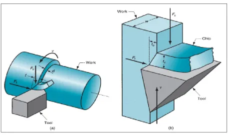
2.3. Forces on Machining

There are two main forces that occur in the machining process, namely F friction force, and N normal force

In Figure 1, we can see the forces in the operating image (a) and orthogonal (b), so that there is a relationship between machining, operating and orthogonal process parameters.

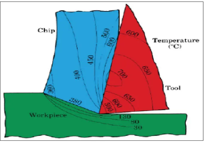
2.4. Cutting Temperature

Almost all of the machining process energy, about 98% (1) was changed to heat. This happens because the high temperature between the chip and the tool is more than 600o_{C, figure 2.}

Cutting temperature is very important because high temperatures can affect:

(1) reduce tool life,

[image:2.595.69.527.341.611.2]

(2) chips become dangerous heat, (3) causing an inaccurate dimension.

[image:3.595.127.469.78.316.2]

Figure 2. Temperature distribution

2.5. Cutting Tool

There are two principle aspects of cutting tools, namely chisel and tool geometry. First the material must have resistance to force, temperature and use in the machining process. Both cutting tools have the optimum geometry between the material and the cutting process.

2.5.1. Tool Life

Tool life is determined by damage to the tool

The mechanism for causing tool damage to the machining process is as follows:

1. Abrasion. It occurs because the chisel particles are carried by material (wear), which causes damage to flank wear.

2. Adhesion. If there are two metal contacts at high Pressures and temperatures, there will be a bond of adhesion or welding occurs between the metals. This happens on the chip and the face of the tool, resulting in erosion / wear on the surface of the tool.

3. Diffusion. Occurs at the boundary between the tool and the chip, causing the surface of the tool to occur hardening. This process occurs continuously, so that the surface of the tool becomes easier to occur abrasion and adhesion damage. Diffusion is the cause of hole damage to the tool, crater wear.

4. Chemical reaction. At high temperatures and high speeds, the surface between the chisel and the chip will occur an oxidation chemical reaction. In this oxide layer new material will occur which will damage the tool.

5. Plastic deformation. Cutting force at the tool angle at high temperatures causes plastic deformation, which makes the tool more susceptible to surface abrasion.

Plastic deformation is a major cause of flank wear. It is important, that the tool damage mechanism is greatly influenced by cutting speed and temperature. The mathematical relationship between cutting speed and tool life is formulated by F.W Taylor, and is called the age equation of Taylor's tool.

𝑣𝑣𝑣𝑣𝑛𝑛_{= 𝐶𝐶 (1)}

Where: v = cutting speed (m / min) T = tool life (minit)

n and C = other parameters, which depend on feeding, depth of cut, work material and chisel.

2.5.2. Sculpture Material

There are several conditions that must be met in the tool material:

1. Toughness. Materials must be resilient to absorb Energy without being damaged, usually a combination of strength and tenacity.

2. Hot hardness. The ability of the material to stay hard at high temperatures.

3. Wear resistance. The ability of the material to resist friction damage, so that the surface of the specimen can be maintained as needed (roughness, smoothness and low friction coefficient).

In general, tool geometry is needed to reduce cutting force, temperature and energy requirements. So that in general it will determine the surface roughness of the turning process.

2.5.3. Effect of Geometry on the Surface

especially radius (NR) and infeed. Is, (a) the surface due to the influence of NR, (b) the effect of the feed, (c) the effect of the cutting angle.

The effect of the tool radius can be combined in the equation, to estimate surface roughness.

𝑅𝑅𝑖𝑖= 𝑓𝑓

2

32𝑁𝑁𝑁𝑁 (2)

Where:

Ri = Average theoretical surface roughness f = feed

NR = Tool Radius at one point. 2.6. Cooling Media

The cooling media has functions including:

1. Reduces friction between debris, chisels and workpieces.

2. Reduces solid temperature and workpiece. 3. Wash flakes

4. Improve surface resolution. 5. Increase tool life.

6. Reduce the power needed.

7. Reduces the possibility of corrosion in workpieces and machinery.

8. Helps prevent sticking of the chisel head.

Cooling media has a condition: does not damage the engine and is stable, has good heat transfer, does not evaporate, is not foamy, provides lubrication and has a high flame temperature. Generally coolers are liquid, because they are easily directed and circulated. Cooling media is very influential on Taylor's tool life, because it can increase the value of C around 10% - 40%. (1)

2.7. Factorial Design

Factorial design is a very important method for determining the influence of several variables that affect results. Conventional experiments only measure one influence of one variable to find out the results. Factorial design can combine several variables in the same factorial test, but it can reduce the number of unnecessary experiments. With factorial design can determine the value of the influence of each variable and the effect of interaction between variables.

2.7.1. Basic Principles

If there are 3 (examples: Temperature T, Concentration C and Catalyst K) variables that will be analyzed, where each variable has 2 specific values (- and +), to determine the effect of each variable, then testing = 23₌₈

So the design factorials:

Temperatur, T (o_{C) Concentration, C (%) Catalyst, K}

- + - + - +

160 180 20 40 A B

With factorial design, 8 trials were obtained (23_=8).

No T C K Test result (example, y %)

1 - - - 60

2 + - - 72

3 - + - 54

4 + + - 68

5 - - + 52

6 + - + 83

7 - + + 45

8 + + + 80

Run

Number TemperatureT (o_C) Concentrati_{on C (%)}

Catalyst

K (A or B)

Results y (%)

1 160 20 A 60

2 180 20 A 72

3 160 40 A 54

4 180 40 A 68

5 160 20 B 52

6 180 20 B 83

7 160 40 B 45

8 180 40 B 80

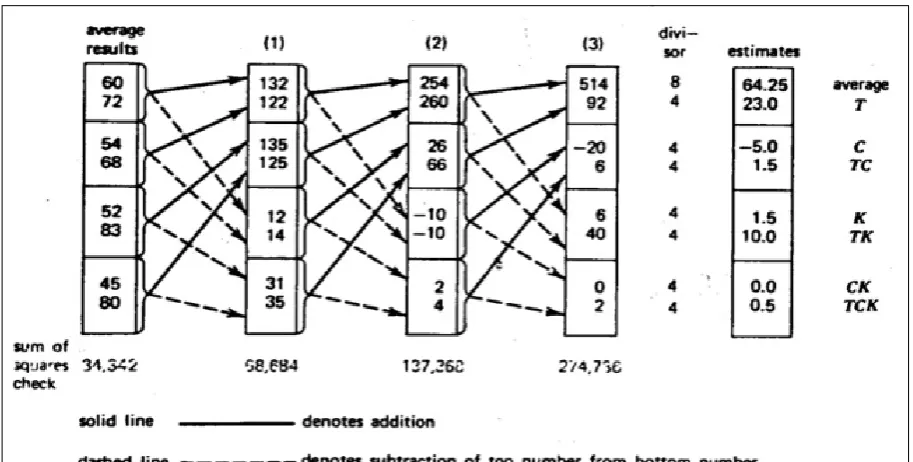
2.8. Algebra Yates's

Algorithm Yates’s is a method for determining the main effects of each variable and the influence of a variable relationship.

[image:5.595.70.527.78.309.2]

Figure 3. Tabulation of the Yates Algorithm

From data processing, the following variables are obtained:

Influence: Temperature, T (o_{C) = 23}o Concentration, C (%) = -5.0 * Catalyst, K (A or B) = 1.5

Temperature (T) + Concentration (C) = 1.5 Temperature (T) + Catalyst (K) = 10o Concentration (C) + Catalyst (K) = 0o T + C + K = 0.5

* Note: The '-' sign indicates the value taken from the bottom value

From processing, the order of the most influential variables is:

Iindividual effect

Temperature Variable = 23o Interaction effect

Temperature + Catalyst variable = 10o

2.9. Least Squares

The Least Squares method is a standard approach for determining equations, if there are several unknown variables. Least Squares is a method of solving by calculating the least number of errors (minimum the sum of errors) of each model of linear equations.

If in an equation there is a value of β's, do not know and the value of x diketahui is known for its value, as the following equation:

(3) Where: β = Constant unknown

x = dominant variable

y = Results of Experiment

After the most influential variable is known, then for 2 data variables (xo and x1), the equation is obtained:

(4) To find the value βo, β1, is to assume the normal distributed equation, namely:

Summing variables (xo, x1 and y) using the Least Square tab.

So the values of βo and β1 are searched by using the matrix.

3. Research Methodology

After getting the test results, then the values of the test results are further evaluated by the Yates ‟algorithm to determine the most influential variables.

1. Determine influential independent variables.

2. Experiment Design.

After determining variables, the author designs an experiment to determine the relationship of these 3 variables. The experimental design uses factorial design, where the writer can determine the number of experiments, namely each variable is carried out by the two limits of the research value, then the number of experiments 23 _{is 8} times the experiment variation. The experiment was done by making a specimen with a lathe process, where previously the variables that would be tested and variables considered constant were previously determined.

3. Testing

Testing is done by measuring the roughness of the results of the turning process from several variations of the experiment. To obtain accurate testing results and can be accounted for, the author conducted a test using a Surfcorder (Surface Rougness Measuring Instrument) at the Center for Metal and Machinery (BBLM) of the Ministry of Industry.

4. Determine the most influential variables.

Test results data is then processed to determine the most influential variables. The test results were processed by using the Yates Algorithm.

5. Determine the correlation of variables.

After obtaining the value of the influential variable, the author determines the mathematical relationship of the variable using the Least Square method.

6. Mathematical Model

The mathematical model was made based on the correlation of the most influential variables, which obtained the function of linear equations that represent variables to surface roughness.

4. Data Collection and Processing

4.1 Data Collection

Research conducted requires machining equipment, materials and testing tools. The data needed to conduct surface roughness testing on the results of the lathe process are as follows:

1. Turning process Lathe specifications

 Type of Lathe Machine: CQ6230A

 Capacity: 150 mm (flashlight distance to bed)  Length: 700 mm (between flashlights)  Manufacturer: Taiwan

2. Cut tool

 Chisel Material: HSS  Dimensions: 3/8 x 4 "Bohler

 Geometric: Angle = 15o_{, Radius = 0.2 mm} 3. Test material, specimen

 Material Type: ST 37

 Tensile Strength: 37 kg / mm2  Violence:

 Elements:

 Diameter, length: L = 20mm; ∅ = 14 mm 4. Cooling media, coolant.

Coolant brand: Castrol Soluble oil, fluid cutting Type coolant: universal Castrol 430 B1

Serial number: no. 2220661 FPC 3402172 5. Surface Roughness Testing

Name of Test Equipment: Surfcorder (Surface Roughness Measuring Instrument) SE 1700α

No. Series: ME X 07636-05 Manufacture: Kosakalab – Japan Test Method: JIS 94

Block Standard: Surface Roughness SS-N model S 94 Ra 3.0µm; No. N21215

4.2. Data Processing

Research carried out based on a predetermined method. 1. Free variable that has an effect

Machining Operations

In conducting surface roughness research, the first step that must be determined will be to collect all the independent variables that affect the surface roughness of the turning process. One of the considerations in determining the independent variable is the mathematical variable in the lathe process.

2. The independent variable in the machining process:  Cutting speed, v (m / s)

 Depth, d (mm)  Feeding, f (mm / min)  Machine capability. Cutting Tool

The tool in the turning process is very influential on the results to be obtained. The first factor is the resistance of the material to the force, temperature and usage during the cutting process. The second factor is the optimum geometry of the tool against the specimen material. Both of these factors determine the roughness of the metal surface. From the results of the experiments that have been carried out, shows that there is a very significant relationship between cutting speed, tool damage, and tool life.

The mathematical relationship between cutting speed with tool life is formulated by F.W Taylor, and is referred to as Taylor's tool age equation. (press. 1).

 Type of Chisel material  Chisel violence  Temperature  Cutting speed  Feeding  Tool life

 Gemetris tool (angle, and tool radius) Specimen Unit

Workpiece materials used will greatly affect surface roughness. This can be seen from the form of growls, chips, which are produced during the machining process. From the results of the tests that have been carried out, there are four types of chips that produce in the machining process, namely:

 Discontinuous chips, which occur in brittle and low speed materials

 Continuous chip occurs in tenacious stamp duty, high speed and small feeding.

 The chip is not broken but there is a deposit (continuous chip with built-up edge), occurs in ductile material and low speed.

 Serrated chips, semi-continuous chips, occur in hard specimen materials and high speeds.

From the study there is a relationship between the types of materials used (ductility and hardness of materials) to surface roughness. The independent variables that affect the roughness of the surface are:

 The type of workpiece used

 Hardness and tenacity of the workpiece Cooling The energy needed in the machining process, about 98% is changed to heat. This happens because the high temperature between the chip and the tool is more than 6000 _{C, (see figure 8). As a result of high heat will cause} damage to the tool, which can ultimately affect surface roughness.

Cooling media is very necessary to reduce and stabilize the strength and hardness of the tool. In some studies cooling media really helped increase the tool life of Taylor from 10% -40%.

From the study, the independent variable that determines the roughness of the surface is the use of cooling media, coolant. From the results of the above study, the independent variables that affect the surface roughness of the turning process are:

 Cutting speed, v  Depth, d  Ingestion, f  Spindle round, n

 Types and materials of sculpture  Chisel hardness

 Temperature  Tool Life

 tool geometry (angle, and tool radius)

 Type of workpiece material

 Hardness and tenacity of the workpiece  Cooling media

Determine the variables to be analyzed

In determining the 3 variables to be analyzed, the authors consider the manufacturing process, time constraints, availability of costs, the results of research that has been conducted, and mathematical studies.

The 3 main variables analyzed are: 1. Spindle rotation, rpm (n) 2. Ingestion, feeding (f) 3. Use of coolant, coolant (C)

Other variables such as geometry and sculpture, geometry and type of material, type and type of lathe, operator, installation and environment are assumed to be constant.

4.3. Experiment Design

Designing experiments based on design factorial methods. Where from the three variables (rotation, feeding, and coolant), 2 testing limits are determined ('-' and '+'), then the design factorial method can be determined by the number of experiments, namely:

Experiment = 2n_,

Where n = number of variables to be tested = 3 (n, f, C)

Experiment = 23 _{= 8}

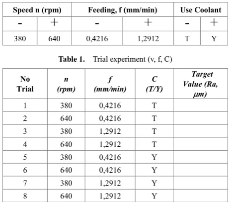
4.3.1. Determine the Test Value

Determining the initial value of testing can basically be arbitrary, so the author determines the value of the test based on the lathe capability, time availability, and cost limitations, the author has set the test value as follows:  Load, n (rpm) = 380 rpm and 640 rpm

 Feeding, f (mm/min) = 0.4216 mm and 1.2912 mm  Using Coolant = using (Y) and not using (T)

So that the initial experimental design becomes:

Speed n (rpm) Feeding, f (mm/min) Use Coolant

-

+

-

+

- +

[image:7.595.305.538.549.752.2]

380 640 0,4216 1,2912 T Y

Table 1. Trial experiment (v, f, C)

No

Trial (rpm) n (mm/min) f (T/Y) C

Target Value (Ra,

µm)

4.3.2. Experiment Process

After determining the value of a variable, as in factorial design, is to determine the preparation for the experiment. Some preparations must be made in the trial process: a. Determine the trial sequence (Run) from the results

of the experimental design.

b. Insert the conditions of lathes, tools and work materials. This is done so that the manufacturing process is carried out with the right process.

c. Perform the turning process stage.

Determining the trial sequence (Run) is very important to ensure that variable changes (n, f, C) do not affect the experimental value and speed up the trial time.

Trial order:

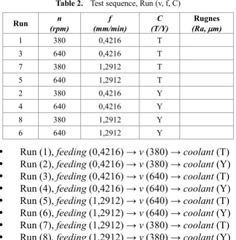
Table 2. Test sequence, Run (v, f, C)

Run _(rpm) n _(mm/min) f _(T/Y) C _(Ra, Rugnes _µm)

1 380 0,4216 T 3 640 0,4216 T 7 380 1,2912 T 5 640 1,2912 T 2 380 0,4216 Y 4 640 0,4216 Y 8 380 1,2912 Y 6 640 1,2912 Y

 Run (1), feeding(0,4216) → v(380) → coolant (T)  Run (2), feeding(0,4216) → v(380) → coolant (Y)  Run (3), feeding(0,4216) → v(640) → coolant (T)  Run (4), feeding(0,4216) → v(640) → coolant (Y)  Run (5), feeding(1,2912) → v(640) → coolant (T)  Run (6), feeding(1,2912) → v(640) → coolant (Y)  Run (7), feeding(1,2912) → v(380) → coolant (T)  Run (8), feeding(1,2912) → v(380) → coolant (Y) 4.4. Surface Roughness

[image:8.595.306.538.221.341.2]

Testing Tests for surface roughness were carried out at the Calibration and Test Laboratory

Table 3. Surface Roughness Test Results

Run _(Rpm) n _(mm/min) F _(T/Y) C

Roughness Test Results, Ra (µm)

1 2 3 Avg 1 380 0,4216 T 3,927 4,003 4,599 4,176 3 64- 0,4216 T 5,928 5,380 6,434 5,914 7 380 1,2912 T 9,541 9,722 9,801 9,688 5 640 1,2912 T 8,354 8,586 8,342 8,427 2 380 0,4216 Y 2,231 2,615 2,953 2,600 4 640 0,4216 Y 2,613 2,908 2,967 2,829 8 380 1,2912 Y 8,106 9,283 8,886 8,758 6 640 1,2912 Y 8,379 8,071 8,966 8,472 Based on the results of Surfcorder testing, Surface Roughness Measuring Instruments, SE 1700α, MIDC -

Bandung)

4.5. Yates's Algorithm

Determining the most influential variables from the results of hardness testing is to use the Yates ‟algorithm.

The results of the turbidity test data are prepared based on the calculations that have been determined in the Yates's Algorithm. (Figure 15)

[image:8.595.58.290.268.504.2]

Calculation of Yates's Algorithm

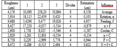
Table 4. Results of Yates' Algorithm Calculations

From the tabulation of Yates's Algorithm, the dominant effect on surface roughness is: 1) Feeding, f = 4,957 µm

4.6. Two Mathematical Variables

After obtaining two dominant variables, then displaying mathematical equations, looking for the values βo and β1, with equation 2.5:

The sum of each variable (xo and x1) is searched by Least Square tabulation.

Table 5. Least Square Tabs

𝛽𝛽0∑𝑥𝑥02+ 𝛽𝛽1∑𝑥𝑥0𝑥𝑥1= ∑𝑦𝑦𝑥𝑥0,

βo(3,690) + β1(1.747,056)= 27,644 (5) 𝛽𝛽0∑𝑥𝑥0𝑥𝑥1+ 𝛽𝛽1∑𝑥𝑥12= ∑𝑦𝑦𝑥𝑥1,

[image:8.595.311.538.525.724.2]

(7)

So by simplifying the matrix (c), then mtrik (c) becomes:

Then: (8)

Then: βo = 5,2024 ; β1 = 0,0048

4.7. Mathematical Model

After knowing the value of βo = 5.2024 and β1 = 0.0048, the mathematical equation mode l of equation 2.4 becomes:

y = 5,2024 xo + 0,0048 x1

xo = feeding variable, f (mm / min)

x1 = rotation variable, n (rpm)Where: y = Surface Roughness, Ra

So that:

Ra = 5,2024 f + 0,0048 n (9) Equation 4.6 applies to boundary conditions:

f = feeding (0,422 -1,291 mm/min) n = speed (380 - 640 rpm)

5. Analysis and Discussion

5.1. Influential Variables

The surface roughness variable that has been processed using the Yates algorithm shows the variation of the effect between the individual effect and the correlation effect, as in table 6.

From table 6, obtained the order of the effect of variables on the roughness of metal surfaces, as follows:

1. Variable rotation n (rpm) = 0.105

This shows that the effect of rotation on the surface roughness in this condition is 0.105 µm. A positive value (+) indicates that the two values of the variable rotation ('-' = 380 and '+' = 640) which affect are at the value of 640

rpm. This shows that high rotation (640) will affect surface roughness value. This is in accordance with the theoretical basis as shown in Figure 11, where tool life is strongly influenced by the high cutting speed, while surface roughness is strongly influenced by tool life.

2. Variable feeding, f (mm / min) = 4,957

This shows that the feeding effect on surface roughness is 4,957 µm. This is the largest value of all variables tested. Positive value (+) shows that 2 feeding variable values ('-' = 0.4216 mm and '+' = 1.2912 mm) which have an effect on feeding 1.2912 mm. This shows that the higher the feeding value will determine the surface roughness value. This is in accordance with the theoretical basis as shown in Figure 14. and equation 2. Where the surface roughness is directly proportional to feeding.

3. Variable Coolant, C (T / Y) = -1,387

This shows that the effect of coolant on surface roughness is -1,387 µm. Negative value (-) indicates that the 2 values of the variable coolant ('-' = 'T' do not use coolant and '+' = 'Y', using coolant) which influence occurs in coolant '-' (T, does not use coolant). This shows that the machining conditions without using coolant will greatly determine the value of surface roughness. This is in accordance with the theoretical basis that almost 98% of the energy used in the metal cutting process is changed to heat. While heat can cause a decrease in tool hardness as shown in Figure 12. Where the higher the heat that occurs, the hardness of the tool will decrease. The decrease in tool hardness will affect the roughness of the metal surface.

[image:9.595.306.535.563.656.2]

Of the three variables analyzed, the feeding variable has the greatest value, this shows that feeding has the greatest influence on the roughness of the metal surface in the turning process, at 4,957 µm. Value '+, shows that roughness occurs at feeding value 1.2912 m / min. It can be said that the greater the feeding, the greater the value of surface roughness.

Table 6. Variation of the effect between the individual effect and the correlation effect

5.2. Mathematical Modeling

[image:10.595.128.471.516.702.2]

Table 7. Least Square tabulation

With this tabulation, the summation results are obtained:

xo2= 3,690 xo.x1= 1.747,056 y.xo= 27,644 x12= 1.108.000 y.x1= 14.446,560

By entering in equation 2.5, it is obtained:

βo (3,690) + β1 (1,747,056) = 27,644

βo (1,747,056) + β1 (1,108,000) = 14,446,560

Then by using a matrix, the values βo and β1 are obtained. Then the mathematical equation model is obtained: Ra = 5, 2024 f + 0,0048 n

With boundary conditions:

f = feeding (0,422 -1,291 mm / min) n = spindle rotation (380 - 640 rpm)

Where surface roughness (Ra) is a function of feeding (f) and rotation (n), 𝑅𝑅𝑎𝑎= 𝑓𝑓(𝑓𝑓, 𝑛𝑛)

With the mathematical equation model, it can be seen graphically the relationship of these variables. From graph it can be seen that the greater the feeding and rotation, the greater the value of roughness.

6. Conclusions and Recommendations

From the results of the metal surface roughness test, the results of the turning process obtained the effect of variables on surface roughness and mathematical model relationships, as follows

6.1. Conclusions

1. The most influential variable on surface roughness is feeding.

2. The biggest surface roughness occurs at conditions f = 1,291mm / min; 640 rpm speed; without cooling media.

3. The mathematical model influences the variable To surface roughness, where roughness is a function of feeding and speed, Ra = f (f, n), are:

Ra = 5, 2024 f + 0,0048 n

Where this equation applies only to conditions: f = (0,422 -1,291 mm / min) and n = (380 - 640 rpm)

6.2. Suggestions

Tests are carried out in conditions of a limited Range of feeding and rotation, so that the mathematical model can only be used in narrow boundary conditions, therefore it is necessary to take further steps:

 Conduct further testing for ranges beyond boundary conditions (feeding and rotation)

 Testing the mathematical model to prove the model.

REFERENCES

[1] Djeffal N., Benslama M., & Messaoudene, I. (2016). Generalized Quantum Key Distribution for WDM Router Applications. Review of Computer Engineering Research, 3(1), 7-12.

[2] Nahar, A. K., Ezzaldean, M. M., Gitaffa, S. A., & Khleaf, H. K. (2016). OFDM Channel Estimation Based on Novel Local Search Particle Swarm Optimization Algorithm. Review of Information Engineering and Applications, 3(2), 11-21.

[3] Mikell P. Groover, "Fundamental of Modern Manufacturing Handbook, Material Process and System", John Wiley & Sons. Inc., 4th edition, New York, 2010, p.443 - 580. [4] Myron L. Begeman, "Manufacturing Process", John Wiley

& Sons. Inc., 8th edition, New York, 1987, p. 449 - 540. [5] Taufiq Rochim, "Specifications, Metrology & Geometric