Extract segmentation lines of 3D model based on minima rule

Journal of Chemical and Pharmaceutical Research, 2014, 6(7):2491-2499

Research Article

_{CODEN(USA) : JCPRC5}

ISSN : 0975-7384

Extract segmentation lines of 3D model based on minima rule

Hui Jia

1,2

, Guohua Geng

1

and Jiangang Zhang

3

1

Dept. of Information Science & Technology, Northwest University, Xi’an, China

2_{School of Computer Science & Technology, Xi’ an University of Posts and Telecommunications, Xi’ an, China} 3_{Information and Supervision Department, Xi’an Thermal Power Research Institute Co Ltd, Xi’an, China}

____________________________________________________________________________________________

ABSTRACT

This paper propose a novel algorithm pipeline to automatically extract the segmentation lines of 3D mesh accurately and efficiently. Our algorithm is based on the minima rule. The minima rule states that human perception usually divides a surface into parts along the concave discontinuity of the tangent plane. The algorithm pipeline has four steps. The first step is the estimate of discrete curvature . The extraction of concave regions of 3D mesh by discrete curvature is the second and critical step; the third step is the thinning algorithm which thin the concave region and eventually got the segmentation lines of 3D mesh; the last step is automatically form a closed loop based on the unclosed segmentation lines around the 3D model. In the end a series of experiments show its accuracy and efficiency.

Keywords: 3D models, minima rule, discrete curvature, concave region, segmentation lines

____________________________________________________________________________________________

INTRODUCTION

3D model segmentation is divided model according to the geometrical characteristics into a set of parts with limited number and each has a simple shape[1]. 3D model segmentation is a research hotspot at present[2,3].The first step of many research methods of works such as model simplification, compression, fast modeling, model deformation, 3D texture mapping, 3D model retrieval is model segmentation. And most of this kind of segmentation is meaningful segmentation[1,5,6], namely according to the minima rule[4], the complex object is as a combination of simple basic elements. Human perception usually divides a surface into parts along the concave discontinuity of the tangent plane. Several approaches have been discussed in the past for decomposing meshes. Aleksey Golovinskiy et al [5] put forward method to mesh partitioning by random cut. The general strategy is to generate a random set of mesh segmentations and then to measure how often each edge of the mesh lies on a segmentation boundary in the randomized set. Kate et al [6] proposed hierarchical mesh decomposition algorithm using fuzzy clustering and cuts. This algorithm proposed a hierarchical mesh decomposition algorithm. First computed decomposition boundary between the components fuzzy. Then, focused on the small fuzzy areas and found the exact boundaries which go along the features of the object. The algorithm also avoided over-segmentation and jaggy boundaries between the components. Halim Benhabiles et al [7] presented automatic 3D-mesh segmentation algorithm based on boundary edge learning. A large database of manually segmented 3D-meshes is used to learn a boundary edge function and a processing pipe line that produce smooth closed boundaries using this edge function was presented. Sun Xiaopeng et al[8] presented a hierarchical mesh segmentation algorithm as semi-supervised k-means clustering and k-ring strip growing. Han Li et al [9] proposed discrete curvature constrained triangle mesh model segmenting technique which is an optimized algorithm. The algorithm classified the vertex attribute based on discrete curvature estimation, and it then combined the region growing method to adaptively determine the topological structure of the 3D models.

The ideas of this article is based on the minima rule from the cognitive theory. The minima rule states that human perception usually divides an object into parts along the concave discontinuity of the tangent plane.

The algorithm consists of four stages:

1.Calculate the discrete curvature. This paper calculated the discrete gaussian curvature and mean curvature of each

vertex of triangular mesh model.

2.Calculate the concave regions of 3D model. According to the model curvature features found concave regions

where segmentation lines located and optimized the concave regions.

3.Region thinning. Calculated edge weight of each edge in concave regions according to the curvature value, utilized

thinning algorithm thinned the concave regions into segmentation lines;

4.Complete segmentation contour. Proposed an automatic contour closing method which completed the segmentation

line to a closed loop around the mesh.

The experimental results prove that this algorithm pipeline can generate more accurate segmentation lines and achieve meaningful segmentation as well. The curvature is calculated once, thinning algorithm is in the concave regions and reduces the calculation range, and contour closing method can achieve accurate results. The algorithm pipeline can improve the efficiency of the extraction of the segmentation line.

EXPERIMENTAL SECTION

Discrete curvature estimation on the point cloud

Scholars have done plenty of studies of the discrete curvature estimation on the point cloud[10,11], among them

Levin[12]put forward curvature estimation algorithm of point sets based on Moving-Least Square Surface（MLS）.

The basic idea is to define the MLS surface

S

as the surface projection ofψ_P, 3

{ | _P( ) }

S= x∈R

ψ

x = x . Directly

compute of surface curvatures for point-set surfaces based on a set of analytic equations derived from MLS. Amenta and Kil[13] gave a more precise definition for projection MLS surfaces as the local minima of an energy function

( , )

e y a

(yis a position vector and a is a direction vector) along the directions given by a vector field

n x

( )

. As shown

in figure 1. Based on this definition, they derived a projection procedure for taking a point onto the MLS surface

S

implied by

n

and

e

, which can be illustrated in Figure 1.

S

is defined as zero solution set of implicit function

g x

( )

。

In the MLS surface, there are three main steps to estimate curvatures of points set. (1) Compute normals of the input points. (2) Project the sample points onto the MLS surface. (3) Compute curvatures of the MLS surface at the projected points. The formulas of computing Gaussian curvature and mean curvature for the implicit surface are

shown as formula 1 and formula 2..

∇

g x

( )

is the gradient of

g x

( )

，

H g x

( ( ))

is the Hessian matrix of

g x

( )

。

Fig. 1 MLS projection procedure

4

( ( )) ( )

det( )

( ) 0

( ) T

G aussian

H g x g x

g x k

g x

∇ ∇

= −

∇

 

 

  ₍₁₎

2

3

( ) ( ( )) ( ) ( ) ( ( ( )))

( ) T

mean

g x H g x g x g x trace H g x g x

k ∇ ∇ − ∇

∇

 

=− 

 

(2)

s

n x

1

j

x+

j

x

0

x

j ( , ( )) e y n x

j

, (x )

j

Calculate the concave regions of 3D model

The different region of 3D mesh

Based on differential geometry knowledge, the concave and convex at some point in curved surface depends on the gaussian curvature K and mean curvature H at that point. Any point in curved surface can be divided into the hyperbolic point (K < 0), parabolic point (K = 0) and elliptic point (K > 0). Due to the existence of noise, only consider the discrete vertex itself does not determine the concave and convex of the region. This paper determines the concave and convex characteristic of a region by the gaussian curvature and mean curvature of the vertex and its neighbors. The concave region can be defined as if the gaussian curvature and the mean curvature of the vertex and its one neighbors are all negative, then this area is concave region.

The algorithm of extracting the concave region

According to the cognitive theory, the segmentation line is located in the minimum negative curvature areas. In order to look for areas of segmentation lines must first find the concave regions, this paper looks for the concave region based on the discrete gaussian curvature and mean curvature of the vertex of the model, in addition cause the discrete curvature is sensitivity to noise, excessive segmentation may appear. In order to further reflect the overall concave areas features in the model surface, region optimization is conducted by region growing and region deleting based on neighborhood area and curvature distribution. After regional optimization, the concave regions can better reflect the regional characteristics of the model. Specific algorithm is as follows:

Input: 3D_point, 3D_face Output: Concave_Region

Step 1: Calculate the gaussian curvature K and mean curvature H of each vertex; Step 2: %Find the vertexes belong to concave regions

Repeat

Step 2.1 find the one neighborhood vertexes

NeiI

of vertex i;

Step 2.2 acquires the gaussian curvature of

NeiI

KN and the mean curvature of vertex i H;

Step 2.3 if KN<0&&H<0 Insert vertex i into Concave_Region

End

Step 3:%region growing Repeat

Step 3.1 Calculate the area value of concave triangles i

concave

A which are formed by one neighbor belongs to vertex i of

Concave_Region;

Step 3.2 Calculate the area value of all triangles i

all

A which are formed by all one neighbors of vertexi;

Step 3.3 if 1

i concave

i all

A

threshold A

≥ ，insert i into Concave_Region。

End

Step 4:%region deleting

Step 4.1 Calculate all connected components of Concave_Region

Step 4.2 Calculate the number of vertexes Vnum_bran and the mean curvature value Gau_bran of each connected component

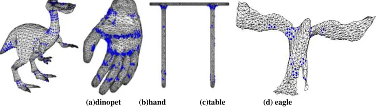
[image:3.595.118.501.641.749.2]

Step 4.3 if Vnum_bran<threshold2 && Gau_bran>threshold3, delete the connected component from Concave_Region

[image:4.595.123.505.86.213.2]

Figure 3 the concave region after regional optimization

Figure 2 shows the concave regions result extracted by step1 and step2, figure 3 shows the ultimate result after regional optimization. In figure 3(a), concave region in neck have been grown, in figure 3(b) concave region in palm have been grown and concave region in wrist have been delete. In figure 3(c) concave region in legs of the table have been delete. In figure 3(d) concave region in the middle of wings have been delete.Threshold is selected by the experiment. Different models have different values because of the Gaussian curvature and mean curvature distribution.

Find the segmentation lines

In this section, we will thin a series of concave region into segmentation lines of the model. Firstly connect the concave area vertex according to the topological relationship into adjacent triangles, and then calculate edge weight according to the curvature values; Secondly classify all the edge into boundary edge set and internal edge set; Thirdly arrange the boundary edge set according to edge weight in ascending order, delete minimum weight boundary iteratively, ultimately thin the concave regions into curves which segment 3D models into parts semantically.

Calculate the edge weight

The edge weight determines whether the edge will be delete or not, need to be calculated in advance. Due to the

segmentation line often appears in the minimum negative curvature region, the edge weight w_l is determined by

curvature. This paper try to use gaussian curvature, mean curvature, maximum principal curvature and minimum principal curvature determine

l

w, finally choose curvature degree value of each vertex which is defined by the average

of maximum minimum principal curvature calculate the vertex curvature, according to the formula (3). In addition discrete curvature is sensitive to noise, in order to more accurately calculate curvature values of the edge, we adopt the

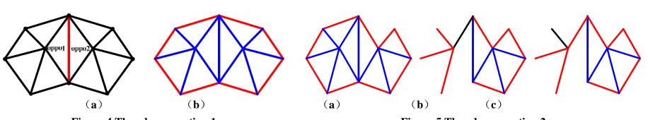
method of figure 4 (a). First calculate the two opposite vertexes of edge l as oppo1

v and oppo2

v ; then calculate two

opposite one neighborsvoppo1 andvoppo2_{. The edge weight of l according to the formula (4), 1k and k2 is the opposite}

one neighbor vertexes number of edgel.

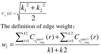
The definition of vertex curvature:

2 2

1 2

(r)

2

v

C

k

k

=

+

（3）

The definition of edge weight：

1 2

1 _ 1_

1 2

1

( )

1

( )

1

2

oppo oppo

ring ring

k k

v v

i i

l

C

r

C

r

w

k

k

=

+

=

=

+

∑

∑

（4）

find the concave region boundary

All the edges of the concave region are divided into two kinds, one is boundary another is the internal edge. The

detection method of boundary is: take an edge e of concave region, e has two adjacent triangles t₁ andt₂. If the

edges of t₁ and t₂ are all belong to the concave region,

e

∉

Boundary

. In contrast if any one edge of t₁ and t₂ does

not belong to the concave region,

e

∈

Boundary

. As shown in Figure 4(b), the red edge is boundary edge, the blue is

internal edge.

[image:4.595.71.238.556.646.2]

[image:5.595.77.535.63.148.2]

（a） （b） （a） （b） （c）

Figure 4 The edge operation 1 Figure 5 The edge operation 2

regional thinning algorithms

Through the edge weight calculation and classify all edge of concave region, the following goal is based on thinning algorithm, after many iterations, thin the concave region into characteristic lines which can represent the region, and have relatively large the sum of edge weight. The method of iterations is constantly deleting the edge which has smallest edge weight. If the deleted edge is belong to the boundary, the deletion will bring edge from internal edge into boundary, as shown in figure 5(a), until the Edge is the empty set, all the edges is belong to the Boundary, the iteration is terminate. During removing connected area need to be guaranteed, in figure 5(b), the black edge should not be deleted while in figure 5(c) the black edge can be deleted. The regional thinning algorithm is shown as follows:

Input: Concave_Region Output: segmentation line

Step 1：%Distinguish between Boundary and Edge

For all e in Concave_Region,

t

₁ and

t

₂ are adjacent triangles of e

If

l

∈ ∨

t

1

t

2

and l∉Concave_ Region

l∈Boundary

Else

l∈Edge

Step 2: %judge and delete e in Concave_Region

While Edge≠ ∅

Step 2.1 List all edges in the Concave_Region by

w

_l in ascending order

Step 2.2 Take out the edge e with smallest

w

_l in Concave_Region

Step 2.3 if

e

∈

Boundary

turn to Step 2.4；

else if e∈Edge

delete e turn to Step 2

Step 2.4

W

_G is the number of connected component before deleted e and

W

_G

'

is after deleted.

If

W

_G

'

>

W

_G %that is to say, delete edgee will make the area disconnected, don't do any operation on edge e . take

the next edge in the sequence as the current edge. Turn to Step 2.3

else

Delete e from Boundary

turn to Step 3

Step 3:% add edge to the Boundary from Edge

Step 3.1 calculate the adjacent line

l

₁and

l

₂of edge e in Concave_Region

Step 3.2 for i=1:2

calculate the adjacent triangles

t

₁ and

t

₂ of

l

_i

while any one lin

t

₁ or

t

₂

l

∉

Concave

_ Re

gion

insert

l

_i into Boundary

turn to Step 2.

end output Boundary。

Regional thinning algorithm has three steps: firstly classify all the edges of Concave_Region into two sets, that is boundary edge Boundary and internal edge Edge. Secondly iteratively delete edge form Concave_Region, the terminal

condition is the Edge is an empty set. When the Edge is not empty, list all edges in the concave_Region by

w

_l in

ascending order, take out edge e which has the smallest

w

_l , if e is in the Boundary, judge whether the edge can be

deleted or not; if e is in the Edge, delete it directly. The condition of e is in the Boundary and can be deleted is after

deletion won't produce new connected component. Thirdly determine which edge in the Edge can be added to the Boundary, and modify Boundary and Edge.

Contour completion

Boundary is as the segmentation line of the 3D model. Most of the time, Boundary is not a closed curve, and need to be

completed and formed a closed loop around the 3D model. Let

β

is selected unclosed segmentation line in Boundary,

the closing process can be defined as iteratively select optimal adjacent point of endpoint of

β

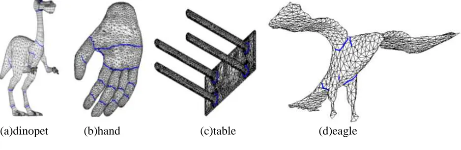
, until a closed loop

around the 3D model is completed. The critical method to form a closed curve is how to find the adjacent vertex which is closest to the most salient feature area. The algorithm from ref.14[14] believe that the user often intends to cut a mesh along boundaries which is perpendicular to the medial axis, but this assumption is not is not suitable to all models. As shown in figure 6. The segmentation lines of the eagle sometimes parallel to the medial axis, such as the line in the wing, sometimes have a certain eagle to the medial axis, such as the line in the legs.

[image:6.595.78.547.340.493.2]

Figure 6 segmentation line

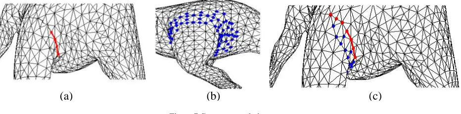
In order to perform automatic contour closing method which completes

β

to a closed loop around the mesh, we use a

method based on combination of multi-feature. The unclosed feature line is coplanar to the closed loop in three-dimensional space, then fitting planar with Constrained Least Squares, then scissor the 3D mesh with the fitting plane. The vertexes which adjacent the intersecting line of the fitting plane with the model can be defined as feasible solution region of the appending vertex. Determine the direction function which can be used to determine the direction of the appending vertex within feasible solution region. There is similarity of curvature characteristic between the appending vertex and the vertex of segmentation line, curve degree characteristic can be used to obtain higher accurate appending vertex.

Feasible solution region Utilize the vertexes of the segmentation line to fit plane. The feasible solution region can be

defined as vertexes set which each vertex has closest distance from vertex to the fitting plane. Let

β

is selected

unclosed segmentation line, n n₁, ₂...n_k are k vertexes of

β

. The plane fitting method utilized the coordinates of these

k vertexes. The general expression for the plane equation is: Ax+By+Cz+ =D 0

(

C≠0

)

,

and A B D

z x y

C C C

= − − − . Note: 0 , 1 , 2

A B D

a a a

C C C

= − = − = − , and z = a x0 +a y1 +a2 . For all k

vertexes

(

k

≥

3)

:

( ,

x y z

_{i i}

, ),

_i

i

=

0,1,

L

,

k

−

1

, utilize points to fit plane, make the formula (5) minimum value.

(

)

1

2

0 1 2

0

n

i i i

i

S

a x

a y

a

z

−

=

=

∑

+

+ −

(5)

In order to make S the minimum value,

0,

0,1, 2

n

s

n

a

∂ = =

∂

. That is to say ：

2

0 2

1

2

i i i i i i

i i i i i i

i i i

x

x y

x

a

x z

x y

y

y

a

y z

x

y

n

a

z

















₌











 





 



∑

∑

∑

∑

∑

∑

∑

∑

∑

∑

∑

. Resolute this system of linear equations, we can get

a

₀

, ,

a a

_{1 2}.

The plane equation is

z

=

a x a y

₀

+

₁

+

a

₂. Let

( , )

i

v i

d

=

dis v z

,if i

v

d

<

ε

, append

v

_i to the feasible solution

region E. As shown in figure 7(a),

β

is the red line, figure 7(b) is the feasible solution region of the contour.

Determine the direction The second feature is determine the direction of the appending vertex. Let

v

p and

v

q are

two endpoint of

β

. Select the one adjacent vertexes

v

₁p_−ring of

v

p within

E

, if

v

q

∈

v

₁p_−ring,then we have found the

loop include

β

; otherwise choose the vertex from

v

₁p_−ring which has closest distance to the fitting plane as the

appending vertex. But this method sometimes can not get the ideal vertex, as shown in figure 7(c), the red points are along the correct direction, but the blue points is wrong although those points have more close distance,thus correct

direction must be defined. Let

cos(

,

)

i

v

v v v v

k p p i

η

=

uuuur uuur

,

v

k

∈

β

,

v

k is adjacent to

v

p.

v

i is adjacent to

v

p too, but

1

i p

ring

v

∈

v

₋ . If

0

i

v

η

>

, the angle between

v v

_{k p}

uuuur

and

v v

_{p i}

uuur

is less than 90 degrees, the direction of

v

i was basically

consistent with

β

, otherwise

v

i is opposite direction.

[image:7.595.74.539.72.173.2]

Figure 7 Contour completion

Curvature characteristic The third feature is the curvature of the appending vertex. Although the appending vertex is

not necessarily belong to the concave area, it always has a large bending degree. The curvature degree value can better

reflect the point bending degree of the model, so according to formula 3 calculate the curvature degree values

c

_v

(r)

of

1

p ring

v

₋ , and get curvature characteristic.

We select among candidate vertexes using the following vertex cost function:

1 2

cos ( )

( )

i

i v v

t v

=

ωη ω



C

r

i

v

∈

E

(6)

1

ω

and

ω

₂ is the weights of directional characteristic

i

v

η

and curvature characteristic

C r

v

( )

, values are normalized

in the range [0:1].

RESULTS AND DISCUSSION

Our segmentation algorithm was evaluated in Windows Operation System, the testing environment is Intel Core i3 3.3GHz CPU, 4G internal memory. In order to compare quantitatively to the most recent algorithms, the Princeton benchmark[15] was used to our 3D-mesh segmentation evaluation. The algorithm include four steps:Calculate the discrete curvature; extract concave region of 3D mesh; find the segmentation lines and contour completion. The figure 2 is the experiment results of the concave region extraction. The blue vertexes are belong to the concave region. The figure 3 shows the concave region after region optimization. According to region grow and region deleting, some vertex is added, some is deleted. Figure 6 shows the segmentation lines after region thinning, according to figure 6, the segmentation lines extracted by our algorithm are all meet the minima rule of visual theory, that is appear in the

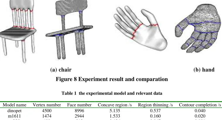
[image:7.595.85.551.359.475.2]

regions of minimum negative curvature. Figure 8 shows the result of contour completion, and the comparison of experiment results with ref. 7. Our algorithm can automatically form a closed loop around the 3D model.

Figure 8(a) our experiment result is similar with ref. 7, in figure 8(b),the segmentation lines extracted by our algorithm is more accurate than ref. 7 and more conducive to hierarchical mesh decomposition. However because of the palm’s bending makes the center of the palm is belong to the concave region, there is a segmentation line located in the center of the palm.In the subsequent work we will use pose-invariant representation to improve. The algorithm of ref. 4 has two steps, the first step is Off-line learning step, The time required for this stage is slightly different because of different learning object, for most of the learning of classification is less than ten minutes. The second step is On-line (segmentation) step, the running time is always within one minute. Our algorithm is automatic segmentation, not required off-line learning. The most time-consuming part of our algorithm is the concave region extraction, which

need to calculate the discrete curvature of every vertex. The time complexity of this step is O( 2

n ), n is the number of

vertex. The time complexity of regional thinning algorithms is O(C),C is the edge number belong to the concave

region, and C<<

n

. The last step is contour completion, which time complexity is depend on the number of vertexes

belong to the feasible solution region E, and E<<

n

. So the time complexity of our algorithm is O(

n

2). The figure 10

is histogram of the relevant experimental data, concave region represent the sum of time of extracting the concave region and regional optimization.

(a) chair (b) hand

[image:8.595.115.494.295.500.2]

Figure 8 Experiment result and comparation

Table 1 the experimental model and relevant data

Model name Vertex number Face number Concave region /s Region thinning /s Contour completion /s

dinopet 4500 8996 5.135 0.537 0.040

m1611 1474 2944 1.533 0.160 0.020

m235 408 812 0.436 0.047 0.001

hand 4696 9388 5.383 0.566 0.042

eagle 1000 1996 0.942 0.096 0.003

table 10082 20160 12.420 1.353 0.086

chair 13463 26926 15.989 1.728 0.093

CONCLUSION

In this paper, we have presented a framework of extraction segmentation lines of 3D model. Based on discrete curvature calculation, we acquired the concave regions of 3D model and conducted the region optimization; according to thinning algorithm, we obtained the segmentation lines of 3D model located in the concave region; finally, under the constraint of fitting plane, we formed a closed loop around the 3D model, achieved the ultimate segmentation of 3D model. Discrete curvature calculation is needed only once for each mesh vertexes and can be performed as preprocessing before the segmentation lines extraction. The experimental results show that the segmentation lines meet the minima rule of the theory of visual, which are located in the smallest negative curvature regions.

[image:8.595.111.499.469.552.2]

Acknowledgments

We gratefully acknowledge the supported by the Natural Science Fund Projects of China(61373117) and the supported by Xian university of posts and telecommunications youth fund(103-0457).

REFERENCES

[1] Shlafman S, Tal A, Katz S. Metamorphosis of polyhedralsurfaces using decomposition [J]. Computer Graphics

Forum, 2002, 21(3): 219-228

[2]Kim V G, Li W, Mitra N J, et al. Learning part-based templates from large collections of 3D shapes J. ACM

Transactions on Graphics (TOG), 2013,32(4): 70.

[3]Wang Y, Asafi S, van Kaick O, et al. Active co-analysis of a set of shapes. ACM Transactions on Graphics (TOG),

2012, 31(6): 165

[4]Hoffman D, Richards W. Parts of recognition . Cognition , 1984, 18.

[5]Aleksey G, Thomas F. Randomized Cuts for 3D Mesh Analysis. ACM Transactions on Graphics (Proc.

SIGGRAPH ASIA) , 2008,27(5).

[6]Katz S, Tal A. Hierarchical mesh decomposition using fuzzy clustering and cuts]. ACM, 2003.

[7]Benhabiles H, Lavoué G et al. Learning Boundary Edges for 3D Mesh Segmentation Computer Graphics Forum, Blackwell Publishing Ltd, 2011, 30(8): 2170-2182.

[8]Sun Xiaopeng, Zhang Qi, Wei Xiaopeng. Semi-supervised 3D Mesh Hierarchical Segmentation. Journal of

Computer-Aided Design & Computer Graphics, 2010,22(04):592-598.

[9] Han Li, Gao Xiaoshan, Chu Bingzhi. Discrete Curvature Constrained Triangle Mesh Model Segmenting

Technique. Journal of Computer-Aided Design & Computer Graphics, 2009,21(06):831-835

[10]Yang P, Qian X. Direct computing of surface curvatures for point-set surfaces// Eurographics symposium on

point-based graphics. The Eurographics Association, 2007: 29-36.

[11]Meyer M, Desbrun M, Schröder P, et al. Discrete differential-geometry operators for triangulated 2-manifolds.

Visualization and mathematics, 2002, 3(2): 52-58.

[12] Levin D. Mesh-independent surface interpolation. Geometric Modeling for Scientific Visualization, 2003, 37-49. [13]Amenta N, Kil Y J. Defining point-set surfaces. ACM Transactions on Graphics (TOG), 2004, 23(3): 264-270. [14]Lee Y., Lee S., Shamir A et al. Mesh scissoring with minima rule and part salience.Computer Aided Geometric

Design , 2005,22, 5 , 444–465. 2, 4,6, 10

[15]Chen X., Golovinskiy A., Funkhouser T. A benchmark for 3d mesh segmentation. ACM Transactions on Graphics