Critical evolution SLO model for single emergencies with multi agents simulation

Journal of Chemical and Pharmaceutical Research, 2014, 6(7):227-238

Research Article

ISSN : 0975-7384

CODEN(USA) : JCPRC5

Critical evolution SLO model for single emergencies with

multi-agents simulation1

Fan Yang and Qing Yang

Wuhan University of Technology Management College, Wuhan University of Technology Huaxia College, China

_____________________________________________________________________________________________

ABSTRACT

Based on the theory of complex systems, and with means of Agent simulation technology, the critical evolution SLO(steady-latent-outbreak state) model and a related simulation model of single emergency is proposed. Research results show that the internal cause of single emergency is the accumulation of internal energy; the evolution is a process from the continuous accumulation of energy to its mass release suddenly. This kind of evolution inevitability could be changed by adjusting inside energy of the system itself or preventing internal transmission action. As the internal transmission action or transfer possibilities are equal to zero, single emergencies could be totally prevented.

Categories and Subject Descriptors: C931; X913.4 [Management]: Management methods

Key words: Single Emergencies, Critical Evolution Mechanism, SLO Model, Cellular Automata, Multi-Agents

Simulation

_____________________________________________________________________________________________

INTRODUCTION

Emergencies such as the East Japan Earthquake, influenza H1N1 and H7N9 raise higher requirements in emergency management. In order to scientifically and effectively conduct active emergency management, we must make clear the evolution mechanism of emergency .According to the system theory, the occurrence of emergencies can be summarized as the interaction of the following three basic factors——human, substance and environment[1,2]. There are two types of emergencies: single emergency and linkage evolution emergency. A single emergency discussed here means the emergency does or assume not bring on other emergencies. The evolution wherever belongs to which type is broadly divided into four phases, the incubation period, the outbreak period, the development period, the recession and dying period[3].

the same evolution rule and updates simultaneously in accordance with certain rule. The simple interaction of a large number of cells constitutes a dynamic and systemic evolution of[6,11].In addition to infectious disease emergencies, models construction for other emergencies can also be used by cellular automaton. Such as: Yassemia etc was designed and implemented forest fire CA model based on geographic information system[12], considering the geological characteristics and factors of fire. Sirakoulis etc, came up CA model (SIR model) for study population movement and the effect of existence of immune to the spread of the disease[13]. On the basis of small-world effect of netizen relationship and network topology, Gensheng Wang[14,15] brought about the orientation-switching rules of netizens’opinions. Likewise, he, in light of small-world network matrix representation of IPO(Internet public opinion) and netizen relationship, constructed evolution and migration model of IPO. Accordingly, by an empirical analysis of the scale-free feature of IPO evolution, he, on one hand, proposed that IPO evolution can be divided into two stages, namely, the viewpoint formation stage and the viewpoint interactive stage. On the other hand, he built up the BA model and put forward the evolution and migration model of IPO characterized by free scale.

Since cellular automata has a distinct advantage in simulating complex systems , when it comes to the event that cannot be solved by conventional mathematical methods, cellular automata offers a better solution[16, 17,18]. Therefore, a comprehensive type of critical evolution SLO model of single emergency is extracted on the basis of other scholars study in this study. It is that the individuals in different emergency are abstracted into intelligent cells, and through the comprehensive analysis of some factors such as cellular neighborhood, transfer probability, transfer amount, system's internal energy etc, the inner factors of single emergency could be digged out. And then two types of evolution of single emergency are implemented through the example cases; extremum and series experiment reconstruct the emergencies scenes. It could provide reference for single emergency management strategy.

1. EVOLUTION MODEL FOR SINGLE EMERGENCY

1.1 Model design

(1) evolution type

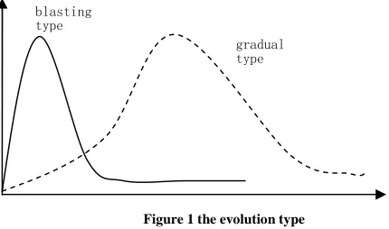
Single emergency in the evolution process can be characterized by two types, one is a blasting type, and the other is a gradual type, as shown in figure 1. Process of the blasting type is shortness, namely lasting time is very short from the happen to a full-blown, and its influence also disappear soon with its full-blown, such as meteor crashed, explosion, etc. The gradual evolution, on the other hand, the internal energy accumulation will take a long time, and once breaking out, it also need a long time to recover, such as H1N1 emergency, etc.

Figure 1 the evolution type

Figure 1 shows the evolution trend of the two types is consistent, just only the speed of evolution is different. So the model design needs to consider the direction of evolution process and the state of each phase of the emergency. And the evolution speed can be adjusted by parameters. Analysis of emergency states is shown in table 1.

Table 1 states analysis for single emergencies

State of Emergencies Illustration

critical point time point of the first individual outbreak

out-break point time point of outbreak individuals number into peak critical state stage between critical point and out-break point period of develop stage after out-break point, yet before declination

period of declination Individuals die or recover, system from a outbreak state into a steady state period of dying out system recovering again

(2) emergencies characteristics and model elements

blasting

type

gradual

______________________________________________________________________________

Through survey of all kinds of single emergencies, the common features are characterized by sudden occurrence, becoming a larger scale in a relatively short time, and propagation individuals in system showed three states: stable, latent and outbreak. Then the analogy, shown in table 2, between emergency characteristics and model elements could be collected by extracting key elements into the important parameters of the model.

Table 2 the analogy between emergencies characteristics and model elements

Reality Systems Simulation System system scale system space: M individual(disseminators or be disseminators, can be people or things) cell Agent individual state (steady, latent, outbreak) cell state days of individual latent latent period: q

individual total duration of outbreak (latent period + outbreak period) the length of cell gene N(A): L(A)

the rate of spread around individuals the possibility of intercellular energy transfer: p0

the ability of individual spread transfer operator: Cij

amount of total individuals of outbreak amount of total cells in outbreak state: f

1.2 Evolutionary Model Implementation

(1) System construction

Assuming that the system is a two-dimensional grid space.，The coordinate of a cellular A_i is (x_i, y_i), i=1,2,…,M，M

is the total of cells. There is one and only one cell A in each unit of grid space. The initial state (t=0) is that all cells are in stable state except one random cell which is in latent state.

Assuming that each cell is communicating and being communicated, energy of adjacent cells in the process of transmission is gradually activated and the total energy of the system will also be gradually accumulated to a critical condition. And a critical state will turn into a chaotic state when a large number of cells outbreak at the same time at a certain point. Then the simulation system outbreaks just like the emergency occurrence.

(2) State parameters

Cell Ai is a dynamics subsystem with certain energy, and its state parameters include cellular gene N(Ai), the energy

value E(Ai), and the current state state(Ai). N(Ai) is the binary number of the specific length L(A), and the location value

of 0 and 1 means stability and disorder respectively. When the sequence of this N(A) full-length is 1, an individual

cell outbreaks; when is 0, it means the steady state; when partially is 1, it means the latent state. The form is as follow:

00000……000 steady state（state=1）

N (Ai)= 11110……000 latent state（state=2） (1)

11111……111 outbreak（state=3）

Changes of its location value indicate the evolution strategy the cellular has taken during the current evolution cycle. The energy E(Ai) of a single cell is determined by the number of 1 in attribute N(Ai), namely

∑

=

=

1 )

(

0

.

1

A i L k k A

n

E

nk is the value of each bit value of N(Ai). Supposing that the value of each bit is 0.1 , the minimum of E(Ai) will be 0

and the maximum 0.1 L(A).

The total energy of the system:

G =

∑

∑ ∑

= = =

=

n

E

1

.

0

(3) Evolution Rule

to “1” .The other way is that the cell can transfer its state to its adjacent cells. cellular in a latent or outbreak state has an impact on the stable cellular ,the latter will become a latent cellular .at the same time, the location value of previous m0 bits of gene N(Aj) will be converted from "0" into "1" (as is described in Chart 1). . Cellular A1 and A6 in

chart 2 are in latent state (others are stable). And Cij represents transfer operator.

Figure 2 Cellular evolution rules

Cell Ai and Aj achieve relevance through a node. Cij denotes the transfer operator with no inverse operator (suppose

sub-association is unidirectional. )

m0 bits 0 changed to1 in N(A) state(A)=1

Cij= (4)

no change state(A)=2 or 3or 0

Cii= add k bits 0 changed to1 in N(A) state(A)=2 and Cij= no change (5)

The evolution of cellular Ai itself can be expressed as:

Cii =the previous k bits of the cellular gene N(Ai)becomes 1,

supposing that state(Ai)=2 and Cji=no change (6)

Note: assuming that k equals 1.

The cell will evolve for T cycles. Each cycle advances step by step according to its evolution rule. The energy of the cellular can be transmitted to each other during the evolution .The possibility of inter cellular energy transfer is p0.

On the other hand, the state of cells may also change, which depends on three factors: energy of neighbor cells, time step and the state of cells in the previous period, among which the possibility of state’s change is p0.

So what can be calculated in each period is:

d: the total number of cells whose state value is 2 f : the total number of cells whose state value is 3

(4) Neighborhood definition

All cells connected with cell(Ai)build up its neighborhood, the cells work only in neighborhood, namely, one cell is

______________________________________________________________________________

Table 3 Neighborhood

A2 (xi, yi + 1)

A3 (xi− 1, yi) Ai (xi, yi) A1 (xi + 1, yi)

A4 (xi, yi − 1)

2. THE CONSTRUCTION AND REALIZATION OF MULTI-AGENT SIMULATION MODEL

The simulation model is based on Multi-Agents in swarm2.2. The term “Agent”, referring to adaptive and autonomous entities, was put forward by Minsky in The Society of Mind which aims to cognize and simulate human intelligence behavior, as follows:

Agent：=｛S_m, Ag_i｝

Sm refers to the Agent internal state while Agi is its function or interaction with the external[19].

This simulation model includes three subjects: Agent Cell A, Agent-model swarm and Agent-environment swarm as table 4. The basic parameters Settings are:

M =worldX×worldY=21×21=441

L(A)=15

Table 4 Agent mapping from The emergency system to the model system

Emergency System Model System

Emergency Environment Environment Agent emergency individual Evolution Agent Monitoring bodies Observer Agent Emergency evolution Model Agent

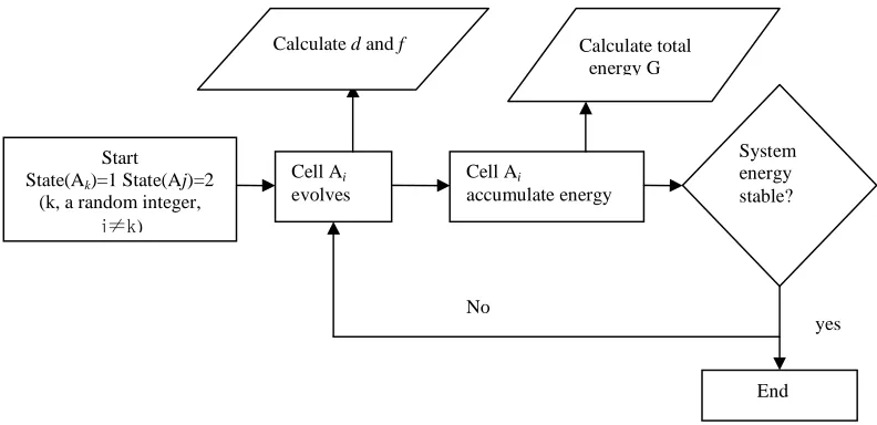
Then, according to simulation algorithm, energy transfer occurs in cell A itself and among cells before the process of emergencies outbreaks being simulated, shown in figure 3.

Figure 3 Simulation flow

3. ANALYSIS OF SIMULATION RESULT

During There are 2 input values : the energy transferring m0 , 0≤m0≤15 (positive integer ) : the possibility of

energy transferring p0 (0≤p0≤1).the greater p0 is ,the higher possibility transferring is successful.

No Start

State(Ak)=1 State(Aj)=2 (k, a random integer,

j≠k)

Cell Ai evolves

Cell Ai

accumulate energy Calculate d and f

System energy stable? Calculate total

energy G

yes

Another three observation values (d.f and G) are also involved in the model : latent value (d), outbreak value (f) and total energy or total destruction (G). Latent value (d) refers to the total of cell A when state(A)=2; and outbreak value

(f) refers to the total of cell A when state(A)=3, total destruction (G) is the total combined energy of cell A at current

cycle.

Besides the three observation values ,we can also study the development process. Suppose when state(A)=1,the

colour is green, when state(A)=2,the colour is yellow, when state(A)=3,the colour is red.

The model expands from its initial state that the state value of a random cell A is 2, and its first bit of gene N(A) is 1.

Experiments conduct 5 times, and the first one as a benchmark experiment could be compared with the others. Experiment 1 and experiment 2 respectively realize the two types of single emergencies: blasting type and gradual type; experiment 2 and 3 are extreme experiment; experiment 4 and 5 consist of a series of experiments.

(1) Experiment 1: Benchmark experiment m0=1 and p0=1

Experiment 1 is a single value experiment. The intercellular transfer is set to be 1, considering the generality of the experiment and highly intensive transferring capacity of unconventional emergencies. The possibility of intercellular energy transfer is also set to be 1, namely, transfer will surely occur. Transfer occurs among all the cells. Each transfer will change some numbers (=m0) of the gene N of a certain cell (state=1) from 0 into 1. The evolution of the

event is shown in figure 4.

t =0 t =13 t =40 t =71

Fig.4. grid of the evolution

Variable t stands for the period of time. The state change indicated that some cells were on the point of breaking out during the 13th period of time when most cells remain stable with minor cells in the latent state. At the 40th period of time, the amount of latent cells reached the maximum and there was a significant increase in the number of out-breaking cells with minor ones stable. By the 71st period of time, all the cells have been breaking out.

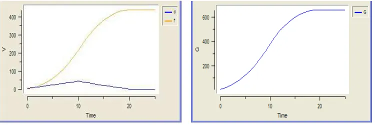
The curves of the other three observed values are shown as follows in Figure 5: Latent value (d), Outbreak value (f) Total destruction (G)

Fig.5. Observation curve (m0=1 and p0=1)

The critical point is set as the time when the first out-breaking point takes place and the moment when latent values reach the maximum is referred to as out-breaking point to which the critical state sustains from critical point. When out-breaking values come to maximum, the full-scale outbreak occurs. By figure 5, the critical state ranged from the

critical point

critical state

outbreak criticaledge

______________________________________________________________________________

13rd period of time to the 40th period of time, accounting for 1/3 of the total period, during which the latent value reaches above the out-breaking value with the internal energy accumulating and the system itself not in the outbreak. By the 40th period of time, the system is on the verge of the critical with the amount of latent cells reaching the maximum. Most cells have undergone the latent state from the starting period to 40th period of time till which the internal energy has achieved to a relatively high level. Since the 40th period of time, the cells began to release the internal energy in a large scale, with the destructive power and outbreak value accelerating their growth. A full-scale outbreak occurred at the 71st period of time. According to the observation, the time lasting from the critical to the outbreak is nearly equal to that from the outbreak to the full-scale one.

This experiment simulated gradual evolution of a single emergency; its results illustrated that the outbreak of emergencies is mainly due to the transfer effect of the inner energy and the accumulation of energy values in the transfer. The entire system is in a critical state after the critical point, and when the energy accumulated to a certain amount, it would change into the out-breaking state at the out-breaking point and remain there until the full-scale outbreak.

(2) Experiment 2: extreme values, m0=14 and p0=1

The aim of this experiment is to test how the evolution will carry out when the output value reaches the maximum. The value of m0 and p0 are set as the maximum, and the initial state of any cell Ai in the system is set as state=2, N(A)

=111111111111110; in other words, the initial cell of the system has reached the extreme, and will transfer the effect to the surrounding in the 100% possibility and at the maximum speed.

Fig. 6.observation curve (m0=14 and p0=1)

As can be seen from the Figure 6, the whole process is shortened from 65 periods of time in the first simulation to 20 periods of time. The out-breaking point when the latent value reaches the maximum 50 is just located at the 10th period of time that is exactly in the middle of the whole process. When the maximum of the latent value falls to 50, there are 21 × 21-50 = 391 cells directly reaches the outbreak state without experiencing the latent state. The result is far above that of the first simulation in terms of both the quantity and the speed and this experiment realizes the blasting process of the single emergency.

(3) Experiment 3: Extreme values m0=0 or p0=0

In contrast with Experiment 2, the purpose of Experiment 3 is to test how the evolution will proceed while the input value is at its minimum. Another extreme case is that one of the input values is 0 or all are 0, which indicates the null transferring effect of the Cell A or the 0 possibility of transfer or the co-existence of the above two circumstances.

Fig.7. Observing curve (m0=0 or p0=0)

The emergency is unlikely to break out when the internal effect and the rate of energy transfer is extremely small in value. In this case, the system is completely stationary and such simple and stable systems are excluded from the consideration.

(4) Experiment 4: series of experiments m0=1 and p0∈(0,1)

Compared with the Experiment 1, this series of experiments aims to investigate the influence of p0’s values on the

evolution result when m0=1 remains unchanged. When p0’s value is set respectively as 0.25, 0.5, and 0.75, the

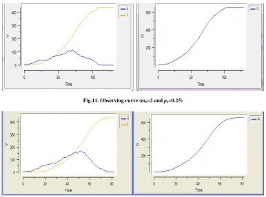
results are shown in Figure 8, 9, 10. In Figure 9, the out-breaking point and the full-scale out-breaking point are both significantly postponed, with the latent values below those in (1). The out-breaking point in the figure is put off to about the 60th period of time and the full-scale outbreak to around the 90th period of time, with the maximum of the latent value is as low as 150. The evolution in Figure 8 and 10 is similar to that of Experiment 1.

Fig.8. Observing curve (m0=1 and p0=0.25)

______________________________________________________________________________

Fig.10. Observing curve (m0=1 and p0=0.75)

As you can see from the three figures, the smaller p0 values slow the speed of the emergency’s occurrence. The

out-breaking point in Figure 8 takes place in the 80th period, later than that in the other cases. In the three cases, there is a significant increase in the number of mutated cells and in the destructive power at the out-breaking point. The smaller the p0 values, the greater the destructive power is. In Experiment 1, the destructive power at the

out-breaking point in the 40th period is around 300, while, the point in Figure 8 stays in the 80th period, that of Figure 9 in the 60th period, that of Figure 10 beyond the 40th period and at the 45th period, with the value of the destructive power all around 500, which indicates the increase of the danger degree of emergency.

(5) Experiment 5: series of experiments m0=2 and p0∈(0,1]

In this series of experiments, the input value of m0 is doubled and the value of p0 is similar with that in Experiment 3,

which aims to observe the effect of the values of p0 on the result of evolution when m0 is valued at 2. The cases of

the four key points p0 = 0.25, p0 = 0.5, p0 = 0.75 and p0 = 1 will be illustrated respectively.

Fig.11. Observing curve (m0=2 and p0=0.25)

In Figure 11, despite the increases in transferring capacity, the transferring possibility decreases. The result of evolution shows that with the maximum of the latent value descending the out-breaking point is put off to around the 70th period, leading to great destructive power at that point. In other words, with relatively low transferring possibility, high transferring capacity leads to greater damage.

The result of this case should have been approaching to that of Experiment 1 in quantity; however, slight differences can be observed in Figure 12. To be specific, the out-breaking point of the system is postponed for 10 periods of time, with the maximal latent value lower than that of Experiment 1.

The increase of the input value m0 accelerates the speed of the effect transfer; and declining the value of p0 in the

meantime that represents the decrease in the possibility of effect transfer, results in the decrease in the latent value and greater damage at the out-breaking point of emergencies. But the full-scale outbreak is not put off and remains at the 80th period with a slight delay. The result also shows that change in the value of p0 plays a greater role than

that of m0.

Fig 13 Observing Curve（m₀=2 and p₀=0.75）

Figure 13 shows that the maximal latent value is greater under the condition that the capacity and possibility of transfer is relatively high. Owing to the high transferring possibility the out-breaking point occurs at the early 40th period with the value of the destructive power at about 400. The system evolution ends in 60th period, lasting a comparatively short term.

Fig 14 Observing Curve（m₀=2 and p₀=1）

Compared with Experiment 1, in Figure 14, with the value of m0 added to 2 and the speed of effect transfer doubled,

the major changes are that the outbreak and the full-scale one both occur 5 weeks ahead of time with the maximal latent value growing a bit. The increase of the value m0 directly accelerates the overall process of the system and

______________________________________________________________________________

CONCLUSION

The results showed that the switch from order to disorder occurred when a certain amount of energy was accumulated and the system was on the brink of the critical point. m0 (the value of inner interaction) and p0 (the possibility value of effect) can impose a great effect on evolution. The reduction of the effect or the prevention of the effect from transferring by isolation might effectively prevent emergencies from happening.

(1) As far as the uncorrelated emergencies are concerned, their evolution rule is that they will definitely break out with a certain amount of energy accumulated inside, which has nothing to do with having or not having an incentive. Out-breaking point might be advanced or postponed based on the transferring forces and the possibility. Being postponed would make the event more dangerous, for the postponed event with a fixed total quantity of energy will break out with greater amount of energy and produce more enormous damage. Therefore, early detection helps control of the event. For instance, if SARS were detected earlier and effectively controlled, it would not have broken out in such a massive pattern.

(2) The effect of the inner transfer is widespread; however, the transferring speed could be checked as possible as it could be. If it (such as earthquake or financial crisis) couldn’t be checked, such measures as isolation can be done to reduce the transfer possibility and also to prevent the occurrence of emergencies to a large extent.

(3)The accumulation of energy will eventually lead to the outbreak of emergencies. The appropriate release of the energy before the out-breaking point may put events under the critical stability. For example, there will not be a mass forest fire if fire is set properly in the forest to release some of its inner energy.

Acknowledgement

This work was supported in part by the Chinese National Natural Science Foundation (No. 91024020), by Humanity and Social Science Youth foundation of Ministry of Education of China (No.14YJCZH165) and by China postdoctoral Fund Projects (No. 2013 M542080).

REFERENCES

[1]Han Zhiyong, Weng Wenguo, Zhang Wei, and Yang Liexun. Scientific background, target and organizational management on major research project MANAGEMENT RESEARCH FOR UNCONVENTIONAL EMERGENCIES Chinese Educational Fund, 2009, 23(4):215-220.

[2]Ma Qingguo, Wang Xiaoyi Major Academic Journal on Management Project，2009，23(3): 126-130.

[3] Fink, S. Crisis Management: Planning for the Inevitable [M]. Lincoln, NE: universe, Inc, 2002. [4] Satsuma J, Willox R, Ramani A, et al. Physica A, 2004, 336(3): 369–375.

[5]Yang Qing, Yang Fan, Journal of Systems Engineering.2012.12.

[6]Li Mingqiang, Zhang Kai, Yue Xiao. Academic Journal of China' University of Economics and Law,2005（6）：

23-26

[7]Xuan HuiYu, Zhang Fa. Simulation and Application of Complex System [M]. Beijing: Tsinghua University Press,

2008

[8]YANG Qing, SHI Yaneng, WANG Zhan. Multi-Agent Research on Immunology-based Emergency Preplan. Proceedings of 2010 International Conference on e-Education, e-Business, e-Management and e-Learning (IC4E 2010) [C]. Published by the IEEE Computer Society，2010:407-410

[9]Khalil, Khaled M., et al. Multi-Agent Crisis Response Systems - Design Requirements and Analysis of Current Systems. Working Paper，2009

[10] Chaczko Z., Moses P. Neuro-Immune-Endocrine (NIE) Models for Emergency Services Interoperatibility. International Conference on “Computer Aided Systems Theory- EUROCAST 2007”[C]. Springer Berlin / Heidelberg，2007:105-112

[11]Qi Huan. Wang Xiaoping. System Modeling and Simulation [M]. Beijing: Tsinghua University Press,2004. [12] Yassemia, S., Dragi ´cevi´ c, S., Schmidt, M. 2008. Ecological Modelling, 2008, 210: 71–84.

[16]Fan Yang, Qing Yang. International Journal of Advancements in Computing Technology. 2012.11. [17]Fan Yang, Qing Yang. Journal of Convergence Information Technology, 2012.12.