Q u a n tifyi n g a n d c o n t e x t u a li si n g
c y clo n e-d r iv e n , e x t r e m e floo d
m a g n i t u d e s i n b e d r o c
k-i nfl u e n c e d d r yl a n d r k-iv e r s
H e r i t a g e , GL, E n t wi s tl e , N S , Mil a n , D a n d Too t h , S
h t t p :// dx. d oi.o r g / 1 0 . 1 0 1 6 /j. a d v w a t r e s . 2 0 1 8 . 1 1 . 0 0 6
T i t l e Q u a n tifyi n g a n d c o n t e x t u ali si n g cy clo n e-d r iv e n , e x t r e m e floo d m a g n i t u d e s in b e d r o c k-i nfl u e n c e d d r yl a n d r iv e r s A u t h o r s H e r i t a g e , GL, E n t wi s tl e, N S , Mil a n , D a n d Too t h , S
Typ e Ar ticl e
U RL T hi s v e r si o n is a v ail a bl e a t :
h t t p :// u sir. s alfo r d . a c . u k /i d/ e p ri n t/ 4 8 8 8 6 / P u b l i s h e d D a t e 2 0 1 8
U S IR is a d i gi t al c oll e c ti o n of t h e r e s e a r c h o u t p u t of t h e U n iv e r si ty of S alfo r d . W h e r e c o p y ri g h t p e r m i t s , f ull t e x t m a t e r i al h el d i n t h e r e p o si t o r y is m a d e f r e ely a v ail a bl e o nli n e a n d c a n b e r e a d , d o w nl o a d e d a n d c o pi e d fo r n o
n-c o m m e r n-ci al p r iv a t e s t u d y o r r e s e a r n-c h p u r p o s e s . Pl e a s e n-c h e n-c k t h e m a n u s n-c ri p t fo r a n y f u r t h e r c o p y ri g h t r e s t r i c ti o n s .
Quantifying and contextualising cyclone-driven, extreme flood
1
magnitudes in bedrock-influenced dryland rivers
2
3
4
GEORGE HERITAGE1, NEIL ENTWISTLE2, *DAVID MILAN3, STEPHEN TOOTH4
5
1 AECOM, Exchange Court, 1 Dale Street, Liverpool, L2 2ET, UK
6
(George.Heritage@Aecom.com)
7
2 University of Salford, Peel Building, University of Salford, Salford, M5 4WT, UK
8
(n.s.entwistle@salford.ac.uk)
9
3 School of Environmental Sciences, University of Hull, Cottingham Road, Hull, HU6 7RX, UK
10
(d.milan@hull.ac.uk)
11
4 Department of Geography and Earth Sciences, Aberystwyth University, Llandinam Building,
12
Penglais Campus, Aberystwyth, SY23 3DB, UK (set@aber.ac.uk)
13
Abstract
15
In many drylands worldwide, rivers are subjected to episodic, extreme flood events and associated
16
sediment stripping. These events may trigger transformations from mixed bedrock-alluvial channels
17
characterised by high geomorphic and ecological diversity towards more dominantly bedrock
18
channels with lower diversity. To date, hydrological and hydraulic data has tended to be limited for
19
these bedrock-influenced dryland rivers, but recent advances in high-resolution data capture are
20
enabling greater integration of different investigative approaches, which is helping to inform
21
assessment of river response to changing hydroclimatic extremes. Here, we use field and remotely
22
sensed data along with a novel 2D hydrodynamic modelling approach to estimate, for the first time,
23
peak discharges that occurred during cyclone-driven floods in the Kruger National Park, eastern
24
South Africa, in January 2012. We estimate peak discharges in the range of 4470 to 5630 m3s-1 for
25
the Sabie River (upstream catchment area 5715 km2) and 14 407 to 16 772 m3s-1 for the Olifants
26
River (upstream catchment area 53 820 km2). These estimates place both floods in the extreme
27
category for each river, with the Olifants peak discharge ranking among the largest recorded or
28
estimated for any southern African river in the last couple of hundred years. On both rivers, the floods
29
resulted in significant changes to dryland river morphology, sediment flux and vegetation
30
communities. Our modelling approach may be transferable to other sparsely gauged or ungauged
31
rivers, and to sites where palaeoflood evidence is preserved. Against a backdrop of mounting
32
evidence for global increases in hydroclimatic extremes, additional studies will help to refine our
33
understanding of the relative and synergistic impacts of high-magnitude flood events on dryland river
34
development.
35
Key words: dryland river, 2D hydraulic modelling, extreme flood, flood estimation, palaeoflood,
36
Sabie River, Olifants River
37
38
INTRODUCTION
40
Drylands (hyperarid, arid, semiarid and dry-subhumid regions) cover 50% of the Earth’s surface and
41
sustain 20% of the world’s population (United Nations, 2016). Many drylands are characterised by
42
strong climatic variations, with extended dry periods interspersed with short, intense rainfall events,
43
and are widely considered to be among the regions most vulnerable to future climate change (Obasi
44
2005; IPCC 2007; Wang et al., 2012). Many dryland river flow regimes are similarly variable
45
(McMahon et al., 1992), with long periods of very low or no flow being followed by infrequent,
short-46
lived, large or extreme flood events (see Tooth, 2013). This variable flow regime is one of the primary
47
controls on dryland river process and form, commonly resulting in channel-floodplain morphologies
48
and dynamics that differ markedly from many humid temperate rivers (Tooth, 2000; 2013; Jaeger et
49
al., 2017). In particular, the role of extreme events in the episodic ‘stripping’ of unconsolidated
50
sediment from alluvial fills on an underlying bedrock template has been reported as a key control on
51
the long-term development of many southern African, Australian, Indian and North American dryland
52
river systems (e.g. Womack and Schumm 1977; Baker 1977; Kale et al. 1996; Bourke and Pickup
53
1999; Wende 1999; Rountree et al. 2000; Tooth and McCarthy 2004; Milan et al., 2018a, Milan et
54
al., 2018b). These stripping events limit long-term sediment build-up and contribute to incremental
55
channel incision over geological time.
56
57
Over the last few decades, research into bedrock-influenced dryland rivers has increased (e.g.
58
Heritage et al., 1999; 2001; Tooth et al., 2002; 2013; Meshkova and Carling, 2012; Keen-Zebert et
59
al., 2013), but hydrological and hydraulic data remain limited owing to the difficulty in collecting
60
information in these typically harsh environments with their relatively infrequent channel-shaping
61
flows. In particular, gauging stations commonly fail to accurately record flow data during large or
62
extreme flood events, as the structures are commonly drowned out and/or suffer physical damage.
63
This paucity of data hampers efforts to develop conceptual and quantitative models of the response
64
of these types of dryland rivers to past, present and future climatic changes, impacting on our
understanding and subsequent management of such systems.
66
67
Similarly, while computational modelling has led to significant insights into the flow hydraulics,
68
sediment dynamics and morphological responses of fully alluvial rivers (e.g. Nicholas et al., 1995;
69
Nicholas, 2005; Milan and Heritage, 2012; Thompson and Croke, 2013), to date there have not been
70
similar advances in our understanding of bedrock-influenced dryland river dynamics. For instance,
71
owing to the paucity of channel roughness information available for these morphologically-diverse
72
river types, past experience has shown that modelling and indirect estimation of extreme discharges
73
commonly has proved problematic and may generate unreliable data (Broadhurst et al., 1997).
74
75
Despite these limitations, improved remote survey technologies and more sophisticated hydraulic
76
modelling software now enhance the possibility of capturing and processing high-resolution
77
topographic data to generate improved estimates of flood hydraulics and magnitudes in
bedrock-78
influenced dryland systems. Against this backdrop, this paper demonstrates how a combination of
79
remotely sensed and field data has been used to apply a 2D hydraulic model for the
bedrock-80
influenced Sabie and Olifants rivers in the Kruger National Park (KNP), South Africa (Fig. 1), where
81
Cyclone Dando generated high-magnitude floods in 2012. Our approach utilised improved data
82
collection, and DEM processing alongside more sophisticated hydraulic modelling and represents a
83
step forward from previous flood modelling estimation work on these rivers that employed 1D
84
modelling (Heritage et al., 2004). The aims are to: 1) use this model to estimate the peak discharges
85
for the floods on these two rivers; 2) compare these estimates with those generated by other
86
commonly-used flood estimation approaches; and 3) compare the estimates with the peak discharges
87
of large or extreme floods recorded or estimated on other southern African rivers. Our approach may
88
be transferable to other sparsely gauged or ungauged rivers that are subject to high-magnitude flood
89
events, and to sites where palaeoflood evidence is preserved, and so may help to refine our
understanding of the magnitude, frequency and impacts of such events on river development.
91
92
STUDY SITES
93
The Sabie and Olifants rivers are located in the southern and central part of the KNP in the
94
Mpumalanga and Limpopo provinces of northeastern South Africa (Fig. 1). The 54 570 km2 Olifants
95
catchment incorporates parts of the Highveld Plateau (2000-1500 m), the Drakensberg Escarpment,
96
and the Lowveld (400-250 m). The 6320 km2 Sabie River covers part of the Drakensberg Mountains
97
(1600 m), the low-relief Lowveld (400 m), and the Lebombo zone (200 m). Rainfall in both
98
catchments is greater in the headwaters (2000 mm yr-1) and declines rapidly eastwards towards the
99
South Africa–Mozambique border (450 mm yr-1). Within the middle reaches, sediment is dominantly
100
sand and fine gravel (median grain size 1-2 mm) (Broadhurst et al. 1997). Although water
101
abstractions have altered the low flows (generally below 50 m3s-1) along both rivers, intermittent
102
cyclone-driven flood flows are unaffected, and the channels remain unimpacted by engineering
103
structures or other human activities over considerable lengths within the KNP. Thus, both rivers
104
represent excellent, near-pristine sites for investigating bedrock-influenced dryland river dynamics.
105
106
Fig. 1.
107
108
In the KNP, both rivers are characterised by a bedrock ‘macrochannel’, which extends across the
109
floor of a 10-20 m deep, incised valley. The macrochannel hosts one or more narrower channels,
110
bars, islands and floodplains (Fig. 2A-C). Outside of the macrochannel, floods have a very infrequent
111
and limited influence. These rivers are characterised by a high degree of bedrock influence, and the
112
diverse underlying geology results in frequent, abrupt changes in macrochannel slope and associated
113
sediment deposition patterns. Locally, bedrock may be buried by alluvial sediments of varying
114
thickness, resulting in diverse channel types that range from fully alluvial (Fig. 2A) to more
bedrock-115
influenced (Fig. 2B-C) (van Niekerk et al. 1995).
117
Fig. 2
118
119
In mid-January 2012, Cyclone Dando impacted on eastern southern Africa. Widespread heavy
120
rainfall (450-500 mm in 48 hours) led to high-magnitude floods along many of the rivers that drain
121
into and through the KNP. Preliminary 2D hydraulic modelling of the Sabie River flood shows that
122
local velocities peaked at 4 ms-1, resulting in extensive erosion and sedimentation along many reaches
123
(Heritage et al. 2014; Milan et al. 2018b). Here, we extend our analyses of the 2012 floods, focusing
124
on the use of a 2D hydrodynamic modelling approach to estimate peak discharges along both the
125
Sabie and Olifants Rivers.
126
127
METHODS
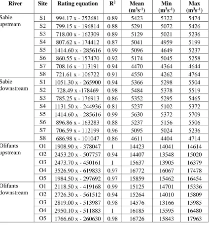
128
Application of a 2D hydrodynamic model requires baseline data on channel topography in the form
129
of a Digital Elevation Model (DEM). Following the Cyclone Dando floods in January 2012, aerial
130
LiDAR and photography (Milan et al., 2018c) were obtained on 30th May 2012 for 50 km reaches of
131
both the Sabie and Olifants rivers in the KNP (Fig. 1). Southern Mapping Geospatial surveyed the
132
rivers using an Opetch Orion 206 LiDAR, flown from a Cessna 206 at 1100 m altitude. Average
133
point density was 409 318 points/km2. The root mean squared error for z was 0.04 m, and for x and
134
y was 0.06 m. Standard deviation for x and y were 0.05 and 0.06 m respectively, based on 5 ground
135
survey points. These data effectively represent the post-flood condition of the rivers, both of which
136
had suffered considerable vegetation and soft sediment stripping. It is argued that this stripping would
137
have occurred up to the peak flood flow and as such this surface would be representative of that which
138
experienced the maximum discharge being estimated in this study.
139
140
Strandline elevations
At selected sites along the Sabie and Olifants rivers, the flow levels associated with the Cyclone
142
Dando floods were surveyed using a Leica 500 RTK GPS in May 2012 (Fig. 1B-C). Despite the four
143
months that had elapsed between the January floods and the surveys (a time gap imposed by the
144
availability of funding), strandlines of organic debris (e.g. branches, twigs, reeds) were very well
145
preserved along significant lengths of each survey reach (Fig. 2E-G). The fresh condition of the
146
debris and occasional ‘best before’ dates on embedded plastic bottles showed clearly that these
147
strandlines were from the January 2012 floods (Fig. 2H).
148
149
Fig. 3.
150
151
Previous work (Heritage et al., 2004; Fisher, 2005) has shown that receding floods can leave several
152
strandlines depending on local conditions. Furthermore, elevation differences of 3 m were often
153
evident between the base and top of individual strandlines, and some strandlines were measured in
154
locations where debris was less abundant than the locations illustrated in Figure 2F-G. Nevertheless,
155
surveys focused on finer organic material such as that showed in Figure 2G, taking the highest
156
elevation debris line as the datum within a given reach, and therefore provide an indication of the
157
highest stage reached by the 2012 floods. Survey of larger woody debris (e.g. Figure 2E) was avoided
158
due to difficulties in determining actual water level given superelevation issues and the flexible nature
159
of the wood.
160
161
Hydrodynamic modelling
162
Post flood LiDAR data (Milan et al., 2018c) for the Sabie and Olifants rivers were used to provide
163
the physical boundary conditions for hydraulic modelling of the 2012 floods. The models represent
164
the longest and most detailed flow simulations conducted on rivers in the region generating hydraulic
165
parameter estimates for the floods at 2 m scale along the 50 km reaches covering a variety of channel
types in single integrated models for each river. Flow resistance parameters are also required to
167
represent many sources of energy loss (Lane and Hardy 2002). A Mannings ‘n’ or Darcy Weisbach f
168
flow resistance value is most often used to represent grain roughness. Previous research protocols
169
have used both a uniform parameter and spatially distributed parameterisation (Legleiter et al. 2011,
170
Logan et al. 2011). Werner et al. 2005 demonstrate that spatially-distributed floodplain roughness
171
failed to improve flood model performance when compared to use of a single roughness class. Horrit
172
and Bates (2002) and Bates et al. (2006) also found that utilisation of a constant channel and
173
floodplain roughness value provided a pragmatic approach to flood modelling. They also note that
174
many of the roughness factors represented by the roughness coefficient in 1D models are integrated
175
into the modelling process in 2D models, most notably form roughness, including the effects of the
176
projection morphological units such as bars and bedrock islands into the flow, which is represented
177
by topographic variation in the DTM and implicitly includes changes in channel type along each 50
178
km modelled reach. As such, no attempt was made to incorporate sophisticated representations of
179
spatial roughness pattern based on factors such as sediment size variation feature types and vegetation
180
community patterns for the study reaches, with a nominal Manning’s ‘n’ roughness value of 0.04
181
used, in the simulations to represent model skin resistance (see Broadhurst et al., 1997).
182
183
JFlow, a 2-D depth-averaged flow model is a commercial 2-D flow modeling tool noted for its ability
184
to handle large data sets through the use of a graphics processing unit-based computation. JFlow was
185
developed as a solution to harness the full detail of available topographic data sets such as those
186
available from LiDAR, and to investigate overland flow paths (Bradbrook, 2006). Simplified forms
187
of the full 2-D hydrodynamic equations are used in the model, but the main controls on flood routing
188
for shallow, topographically driven flow are captured (Bradbrook, 2006). As such JFlow simulations
189
must be regarded as only a first approximation of 2D flow but its ability to handle topographically
190
induced form roughness (a major resistance component on the systems being studied) and its
relatively rapid run time and robustness on long complex reaches makes it ideal for the proposed
192
modelling .The model also performed well compared to other shallow water simulations in a
193
benchmarking exercise by the EA (Néelz, & Pender, 2013). Bates et al. (2010) and Neal et al. (2010)
194
demonstrated that the model was capable of simulating flow depths and velocities within 10% of a
195
range of industry full shallow water codes such as TuFlow and InfoWorks. Their simulations of
196
gradually varying flows, revealed that velocity predictions were ‘surprisingly similar’ between the
197
models and they suggest that JFlow model may be appropriate for velocity simulation across a range
198
of gradually varied subcritical flow conditions.
199
200
The DEMs of each study reach were degraded to uniform 1 m data grids and input into the JFlow
201
software to generate 2 m resolution surface meshes using a uniform triangulation algorithm.
202
Morphologic scale form roughness variation (and by definition channel type) was defined using the
203
local bed level variation derived from the original survey data (see Entwistle et al., 2014). It was
204
assumed that at the flow peak the majority of the soft sediment and vegetation in the two rivers had
205
been eroded, as such their impacts on flow resistance were not considered.
206
Inflow and outflow discharges and flow stage boundaries were set during hydraulic model runs, based
207
on low flow survey data and high flow approximations (these were refined within the program during
208
model runs to satisfy the conservation of mass and momentum equations). Flow simulations were
209
conducted up to 5000 m3s-1 on the Sabie River and 15 000 m3s-1 on the Olifants River. These upper
210
values were chosen based on a continuity equation estimate of peak flows, which was undertaken
211
whilst in the field. These data were used to develop simulated rating curves for each of the study
212
sites.
213
214
Flood estimation
215
Simulated water surface elevation versus simulated discharge rating curves were derived for the
216
upstream and downstream parts of each of the sites shown in Fig. 1. These values were used to
estimate peak flows using the surveyed RTK GPS strandline elevations.
218
219
RESULTS
220
Model validation
221
Comparisons were made between the simulated water surface elevations and the RTK GPS surveyed
222
strandlines (Fig. 3). For the Sabie (Fig. 3A), very close matches were found at sites 1, 2, 4 and 6,
223
with RTK elevations mostly within 0.3 m of the simulated water elevations. Simulated water
224
elevations are over-predicted by 0.5-1.5 m for sites 3 and 5, whereas simulated water elevations were
225
under-predicted by 1.0-1.5 m at sites 7 and 8 farther downstream. For the Olifants (Fig. 3B),
226
simulated water surfaces show much more variability but surveyed strandline elevations are generally
227
within 1 m of the simulated elevations The water surface simulation data suggest that the assumptions
228
of gradually varied flow and subcritical flow are not always satisfied along the model reaches
229
(Coulthard et al., 2013) and this will introduce a degree of error in the calculated discharges. For
230
both rivers, the deviation between simulated and measured elevations was in the same order as the
231
vertical variation ( 3 m) evident for the strandlines (Fig. 2). Some parts of the surveyed elevations
232
along the strandlines matched simulated water elevations better than others, suggesting the possibility
233
of multiple strandlines having been surveyed. Although we are unable to substantiate, this may result
234
from pulsing or recession of flood peaks. This could not be verified due to a lack of gauge data for
235
the flood. Modelled and surveyed flood inundation extents are also plotted in Fig. 4. For the Sabie
236
River, there is a very close match between modelled and surveyed inundation extents (Fig. 4A),
237
whereas for the Olifants River, simulated flood extent appears to be slightly under-predicted (Fig.
238
4B).
239
240
Fig. 4.
241
Extreme flood estimation
243
The highest simulated flood stage of 5000 m3s-1 for the sites along the Sabie River is lower in
244
elevation than the majority of strandline measurements and does not exceed the surveyed limits of
245
the flood extents (Fig. 4A). This suggests that during the 2012 floods, peak discharges were slightly
246
in excess of this simulated flow. Regression analysis-derived rating equations for each study site
247
along the Sabie study reach (Fig. 1B) allowed estimation of the peak flood magnitude, which ranges
248
from 4470 m3s-1 to 5630 m3s-1 (Table 1, Fig. 5). For the Sabie River, these results suggest that 2012
249
flood did not exceed the peak stage or extent of the 2000 Cyclone Eline floods, which ranged between
250
6000 and 7000 m3s-1 towards the lower end of the Sabie study reach (Heritage et al., 2003). This
251
conclusion is supported by field observations from the Sabie River. At the Low Level Bridge crossing
252
near Skukuza (Fig. 1A), a roadside marker indicates the limit of the 2000 floods. This marker stands
253
at a higher elevation than the strandlines from the 2012 floods, indicating that at this location, the
254
2012 floods were not as large as the 2000 flood event. The anecdotal accounts of park rangers suggest
255
that this finding also applies more widely along the Sabie study reach, and is supported by the absence
256
of any damage during the 2012 floods to the tarred road that runs adjacent to the macrochannel
257
margins along the right bank, where comparatively this road had been extensively damaged during
258
the 2000 event.
259
260
Table 1.
261
262
Fig. 5.
263
264
The 15 000 m3s-1 flood simulation for the sites along the Olifants River exceeds some of the surveyed
265
strandline elevations but remains within the limits of the surveyed flood extents (Fig. 3). This
266
suggests that during the 2012 floods, peak discharges approached or slightly exceeded this simulated
267
flow. Regression analysis derived rating equations for each study site allowed estimation of the peak
flood magnitude, which ranges from 14 407 m3s-1 to 16 772 m3s-1 depending on location (Table 1,
269
Fig. 5).
270
271
DISCUSSION
272
Comparisons between flood estimation methods
273
The method used in this paper to estimate flood magnitudes along the Sabie and Olifants rivers can
274
be compared to other published methods for estimating (palaeo) flood velocities and discharges.
275
These range from the use of regime type equations (e.g. Wohl and David, 2008), maximum
276
transported grain size and/or bedform dimensions (e.g. Costa, 1983; Williams, 1983; Wohl and
277
Merritt, 2008) and friction based approaches (e.g. Kochel and Baker, 1982; Heritage et al., 1997;
278
Broadhurst et al., 1997; Birkhead et al., 2000).
279
280
Wohl and David’s (2008) width–discharge relationship for bedrock-influenced channels is
281
statistically significant, but the r2 value for the regime equation was low at 0.59, principally due to
282
variation in rock strength. This relationship was applied to the study sites on the Sabie and Olifants
283
rivers (Fig. 2) and generated peak flows of between 25 000 to 50 000 m3s-1 for the Sabie
284
(macrochannel width 250-500 m), and 75 000 m3s-1 in wider reaches on the Olifants (macrochannel
285
width 700 m). All but the lower values are outside the range of data used by Wohl and David (2008)
286
to generate the original width–discharge relationship. As such, little confidence can be placed in the
287
application of this regime type approach to estimating flood magnitude on the KNP rivers.
288
289
Application of the maximum transported grain size to derive an average flood velocity estimate
290
(Costa, 1983; Williams, 1983) is also difficult to apply in the case of the Sabie and Olifants rivers.
291
In both catchments, the metamorphic and igneous bedrock weathers to supply mainly sand and fine
292
gravel (granules, minor pebbles) to the rivers. Consequently, cobble- or boulder-sized sediment is
supply limited and any use of the empirical relationships would lead to a gross underestimation of
294
peak discharges.
295
296
Application of the slope-area method to the downstream parts of the study reaches of both rivers using
297
an estimated Darcy-Weisbach friction factor of 0.125 and a strandline-derived macrochannel water
298
surface slope generated peak discharge estimates of between 3112 m3s-1 and 3558 m3s-1 for the Sabie
299
River and between 12 923 m3s-1 and 13 417 m3s-1 for the Olifants River. These estimates are lower
300
than the peak discharge predicted using the 2D modelling approach and are likely to be less accurate
301
as the technique utilises an average reach slope and estimated roughness coefficients derived from
302
the strandline data and previously published research (Broadhurst et al., 1997; Birkhead et al., 2000).
303
This contrasts with the 2D approach adopted here where the form roughness and water surface slope
304
are intrinsically linked to the detailed local topographic variation captured in the baseline digital
305
elevation model.
306
307
In summary, these alternative approaches to flood discharge estimation along the Sabie and Olifants
308
rivers yield a wide variety of values, with some approaches clearly inapplicable or inappropriate given
309
the context of the study sites. Even the more sophisticated approaches that utilise slope, area and
310
friction data require many of these parameters to be estimated or are limited by difficulty in accurately
311
measuring strandlines in the field.
312
313
The simplified 2D JFlow method applied in this study does not require such data and can estimate
314
flood discharge from a detailed topographic model alone (e.g. a LiDAR-derived DEM). This model
315
contains ‘effective’ parameters that are related to aggregated hydraulic processes, which cannot, in
316
general, be determined from the physical characteristics of the reach under consideration (Hunter et
317
al., 2007). Channel form roughness, capturing protrusion into the flow at the morphological unit scale
318
(including sand bars, bedrock islands etc. which when aggregated also represent channel type
differences), is explicitly integrated into the modelling approach through the detailed LiDAR DEM
320
and, as outlined earlier, for our study a single representative grain and hydraulic flow resistance value
321
was input to the model as this represents only a minor component of flow resistance. Stripping of
322
vegetation and soft sediment was also likely to have occurred up to the peak discharge and as such
323
the stripped DEM surveyed after the floods was assumed to adequately represent the overall form
324
resistance operating at the flood peak.
325
326
Previous research (e.g. Werner et al., 2005) supports this approach, demonstrating that
spatially-327
distributed floodplain roughness based on land-use mapping failed to improve flood model
328
performance when compared to use of a single floodplain roughness class. Horrit and Bates (2002)
329
and Bates et al. (2006) also found that utilisation of a constant channel and floodplain roughness value
330
provided a pragmatic approach to flood modelling. Such an approach is also justified on the premise
331
that the approach is primarily for use in estimating palaeofloods. As such, in these previous studies
332
no attempt was made to incorporate more sophisticated representations of spatial roughness pattern
333
based on factors such as sediment size variation and vegetation community patterns, as these data are
334
typically not available in palaeocontexts.
335
336
Comparisons with extreme floods on other southern African rivers
337
Based on the historic flow record (Fig. 6A), the 2012 Cyclone Dando flood on the Sabie River can
338
be classed as ‘extreme’. As noted, however, this was a smaller magnitude flood than the 2000 flood
339
event (Heritage et al., 2004) and a detailed comparison shows that the 2012 event overall had a more
340
subdued morphological impact (Milan et al., 2018b). Based on the historic record (Fig. 6B), the 14
341
407 m3s-1 to 16 772 m3s-1 flood estimate for the Olifants River appears to be more extreme. Indeed,
342
in comparison with the catalogue of maximum peak discharges compiled by Kovacs (1988) and other
343
related studies, this 2012 event ranks among some of the most extreme floods recorded for any
southern African river in the last couple of hundred years (Fig. 7). For instance, the 2012 Olifants
345
River flood far exceeds the well-documented 1981 Buffels River flood of up to 8000 m3s-1 (Stear,
346
1985; Zawada, 1994), the 1987 lower uMgeni River flood of 5000-10 000 m3s-1 (Cooper et al., 1990;
347
Smith, 1992) and the 1974 and 1988 discharges of 8000-9000 m3s-1 that occurred along the much
348
larger middle Orange River (du Plessis et al., 1989; Bremner et al., 1990; Zawada and Smith, 1992;
349
Zawada, 2000). The 2012 Olifants River flood is even comparable in magnitude to the extreme floods
350
that occurred along rivers draining to the KwaZulu-Natal coast during Cyclone Domoina in January
351
1984 (Kovacs et al., 1985; Kovacs, 1988). Higher discharges have almost undoubtedly occurred
352
along much larger rivers such as the Orange earlier in the Holocene; for example, 13 palaeofloods
353
with discharges in the range of 10 000-15 000 m3s-1 occurred along the lower Orange River during
354
the last 5500 years and were exceeded by one catastrophic discharge of around 28 000 m3s-1
355
sometime between AD 1453 and AD 1785 (Zawada 1996; 2000; Zawada et al., 1996). Nevertheless,
356
the Olifants River flood remains notable on an historic timescale, particularly given the associated
357
geomorphological impacts, which involved widespread stripping of alluvium along extensive reaches
358
of the river in the KNP (Fig. 2D).
359
360
Fig. 6.
361
362
Fig. 7.
363
364
365
CONCLUSION
366
In this paper, a simplified 2D modelling approach has been used to estimate the magnitudes of the
367
cyclone-driven, flood events on the Sabie and Olifants rivers in January 2012. The method relies on
368
an accurate LiDAR-derived DEM of a river to account for form roughness assuming that vegetation
369
and soft sediment stripping had occurred prior to the flood peak, and applies a uniform additional
roughness factor to account for grain and hydraulic flow resistance components. The use of a
371
simplified 2D code allows for more rapid simulations, modelling very large areas in detail and
372
provides a robust modelling framework that can generate hydraulic estimates for a range of flows.
373
Comparison of field surveyed and simulated water surface slope and inundation patterns for the peak
374
flows suggests that the model performs well overall.
375
376
On both rivers, the flood flows can be described as ‘extreme’, with the discharge on the Olifants being
377
among one of the largest ever recorded or estimated for any southern African river in the late
378
Holocene. Given the documented changes in rainfall patterns in the Kruger National Park since the
379
1980’s (MacFadyen et al., 2018) whereby seasonal patterns appear to be attenuating and rainfall
380
extremes on both ends of the spectrum appear to be extending it is possible that flood extremes on
381
the two study rivers and other systems on the region are becoming increasingly likely. On systems
382
where such extremes are known to drive geomorphic change (Milan et al., 2018b) this may trigger a
383
state change towards bedrock-dominated systems, illustrating the impact of climate change on the
384
region.
385
386
387
ACKNOWLEDGMENTS
388
This project was funded through NERC Urgency Grant NE/K001132/1. We would like to thank
389
SANParks for supporting this research. JBA Consulting are acknowledged for allowing use of JFlow.
390
391
REFERENCES
392
Baker, V.R., 1977. Stream-channel response to floods, with examples from central Texas. Geological
393
Society of America Bulletin 88, 1057-1071.
394
Bates, P.D., Wilson, M.D., Horritt, M.S., Mason, D.C., Holden, N., Currie, A., 2006. Reach scale
floodplain inundation dynamics observed using airborne synthetic aperture radar imagery: Data
396
analysis and modelling. Journal of Hydrology 328, 306-318.
397
Bates, P.D., Horritt, M.S. and Fewtrell, T.J., 2010. A simple inertial formulation of the shallow water
398
equations for efficient two-dimensional flood inundation modelling. Journal of Hydrology,
387(1-399
2), pp.33-45.
400
Birkhead, A.L., Heritage, G.L., James, C.S., Rogers, K.H., van Niekerk, A.W., 2000.
401
Geomorphological change models for the Sabie River in the Kruger National Park. Water Research
402
Commission Report 782/1/00.
403
Bourke, M.C., Pickup, G., 1999. Fluvial form variability in arid central Australia. In: Miller, A.J.,
404
Gupta, A. (Eds), Varieties of Fluvial Form. Chichester: Wiley, pp. 249-271.
405
Bremner, J.M., Rogers, J., Willis, J.P., 1990. Sedimentological aspects of the 1988 Orange River
406
floods. Transactions of the Royal Society of South Africa 47, 247–294.
407
Bradbrook, K., 2006. JFlow: a multiscale two‐dimensional dynamic flood model. Water and
408
Environment Journal, 20(2), pp.79-86.
409
Broadhurst, L.J., Heritage, G.H., van Niekerk, A.W., James, C.S, Rogers, K.H., 1997. Translating
410
discharge into local hydraulic conditions on the Sabie River: an assessment of channel flow
411
resistance. Water Research Commission Report 474/2/97.
412
Cooper, J.A.G., Mason, T.R., Reddering, J.S.V., Illenberger, W.K., 1990. Geomorphic effects of
413
catastrophic flooding on a small estuary. Earth Surface Processes and Landforms 15, 25-41.
414
Costa, J.E., 1983. Paleohydraulic reconstruction of flash-flood peaks from boulder deposits in the
415
Colorado Front Range. Geological Society of America Bulletin 94, 986-1004.
416
Coulthard, T.J., Neal, J.C., Bates, P.D., Ramirez, J., Almeida, G.A. and Hancock, G.R., 2013.
417
Integrating the LISFLOOD‐FP 2D hydrodynamic model with the CAESAR model: implications
418
for modelling landscape evolution. Earth Surface Processes and Landforms, 38(15),
pp.1897-419
1906.
420
du Plessis, D.B., Dunsmore, S.J., Burger, C.E., Randall, L.A., 1989. Documentation of the February–
March 1988 floods in the Orange River basin. Pretoria: Department of Water Affairs, Technical
422
Report TR 142.
423
Entwistle, N.S., Heritage, G.L., Tooth, S., Milan, D., 2014. Anastomosing reach control on hydraulics
424
and sediment distribution on the Sabie River, South Africa. Proceedings of the International
425
Association of Hydrological Sciences 367, 215-219.
426
Fisher, T.G., 2005. Strandline analysis in the southern basin of glacial Lake Agassiz, Minnesota and
427
North and South Dakota, USA. Geological Society of America Bulletin 117, 1481-1496.
428
Heritage, G.L., Large, A., Moon, B., Jewitt, G., 2004. Channel hydraulics and geomorphic effects of
429
an extreme flood event on the Sabie River, South Africa. Catena 58, 151-181.
430
Heritage, G.L., Large, A.R.G., Moon, B.P., Birkhead, A.L., 2003. Estimating extreme flood
431
magnitude in bedrock-influenced channels using representative reach-based channel resistance
432
data. Geografiska Annaler: Series A, Physical Geography 85, 1-11.
433
Heritage, G.L., Moon, B.P., Jewitt, G.P., Large, A.R.G., Rountree, M., 2001. The February 2000
434
floods on the Sabie River, South Africa: an examination of their magnitude and frequency. Koedoe
435
44, 37–44.
436
Heritage, G.L., Tooth, S., Entwistle, N., Milan, D.J., 2014. Long-term flood controls on semi-arid
437
river form: evidence from the Sabie and Olifants rivers, eastern South Africa. Proceedings of the
438
International Association of Hydrological Sciences 367, 141-146.
439
Heritage, G.L., van Niekerk, A.W., Moon, B.P., 1999. Geomorphology of the Sabie River, South
440
Africa: an incised bedrock-influenced channel. In: Miller, A.J., Gupta, A., (Eds.), Varieties of
441
Fluvial Form: Wiley, Chichester, pp. 53–79.
442
Heritage, G.L., van Niekerk, A.W., Moon, B.P., Broadhurst, L.J., Rogers, K.H., James, C.S., 1997.
443
The geomorphological response to changing flow regimes of the Sabie and Letaba river systems.
444
Report-Water Research Commission, vol. 376/1/97. Pretoria, South Africa. 164 pp.
445
Horritt, M.S., Bates, P.D., 2002. Evaluation of 1D and 2D numerical models for predicting river flood
inundation. Journal of Hydrology 268, 87-99.
447
Hunter, N.M., Bates, P.D., Horritt, M.S., Wilson, M.D., 2007. Simple spatially-distributed models
448
for predicting flood inundation: a review. Geomorphology 90, 208-225.
449
IPCC., 2007. Climate Change 2007: Synthesis Report. Summary for Policymakers. IPCC.
450
Jaeger, K.L., Sutfin, N.A., Tooth, S., Michaelides, K., Singer, M., 2017. Geomorphology and
451
sediment regimes of intermittent rivers and ephemeral streams. In: Datry et al. (Eds.), Intermittent
452
Rivers and Ephemeral Streams: Ecology and Management, Elsevier, in press.
453
Kale, V.S., Baker, V.R., Mishra, S., 1996. Multi-channel patterns of bedrock rivers: an example from
454
the central Narmada basin, India. Catena 26, 85–98.
455
Keen-Zebert, A., Tooth, S., Rodnight, H., Duller, G.A.T., Roberts, H.M., Grenfell, M., 2013. Late
456
Quaternary floodplain reworking and the preservation of alluvial sedimentary archives in
457
unconfined and confined river valleys in the eastern interior of South Africa. Geomorphology 185,
458
54-66.
459
Kochel, R.C., Baker, V.R., 1982. Paleoflood hydrology. Science 215, 53-361.
460
Kovacs, Z.P., 1988. Regional Maximum Flood Peaks in Southern Africa. Pretoria: Department of
461
Water Affairs, Directorate of Hydrology, Technical Report 137.
462
Kovacs, Z.P., du Plessis, D.B., Bracher, P.R., Dunn, P., Mallory, G.C.L., 1985. Documentation of the
463
1984 Domoina floods. Pretoria: Department of Water Affairs, Technical Report TR 122.
464
Lane, S.N., Hardy, R.J., 2002. 16-Porous rivers: A new way of conceptualising and modelling river
465
and floodplain flows? Transport Phenomena in Porous Media II, 425-449.
466
Legleiter, C.J., Kyriakidis, P.C., McDonald, R.R. and Nelson, J.M., 2011. Effects of uncertain
467
topographic input data on two‐dimensional flow modeling in a gravel‐bed river. Water
468
Resources Research, 47(3).
469
Logan, B.L., McDonald, R.R., Nelson, J.M., Kinzel, P.J. and Barton, G.J., 2011. Use of
470
multidimensional modeling to evaluate a channel restoration design for the Kootenai River, Idaho
471
(No. 2010-5213, pp. i-68). US Geological Survey.
McMahon, T.A., Finlayson, B.L., Haines, A.T., Srikanthan, R., 1992. Global runoff: continental
473
comparisons of annual flows and peak discharges. Catena Paperback. Cremlingen-Destedt.
474
MacFadyen, S. , Zambatis, N. , Van Teeffelen, A. J. and Hui, C. 2018. Long‐term rainfall regression
475
surfaces for the Kruger National Park, South Africa: a spatio‐temporal review of patterns from
476
1981 to 2015. International Journal of Climatology, 38: 2506-2519.
477
Meshkova, L.V., Carling, P.A., 2012. The geomorphological characteristics of the Mekong river in
478
northern Cambodia: a mixed bedrock–alluvial multi-channel network. Geomorphology 147–148,
479
2–17.
480
Milan, D.J., Heritage, G.L., 2012. LiDAR and ADCP use in gravel bed rivers: Advances since GBR6.
481
In Church, M., Biron, P., Roy, A., (Eds.), Gravel-bed rivers: Processes, Tools, Environments.
482
John Wiley & Sons, Chichester, p. 286-302.
483
Milan, D., Heritage, G., Entwistle, N. and Tooth, S., 2018a. Morphodynamic simulation of sediment
484
deposition patterns on a recently stripped bedrock anastomosed channel. Proceedings of the
485
International Association of Hydrological Sciences, 377, p.51.
486
Milan, D.J., Heritage, G.L., Tooth, S., Entwistle, N., 2018b. Morphodynamics of bedrock-influenced
487
dryland rivers during extreme floods: insights from the Kruger National Park, South Africa.
488
Geological Society of America Bulletin.
489
Milan, D.J., Heritage, G., Tooth, S. 2018c. Kruger National Park Rivers LiDAR data 2012. Centre
490
for Environmental Data
491
Analysis. http://catalogue.ceda.ac.uk/uuid/a2e82c7f92dc4f389a7fb7e4e6629c9e
492
Neal, J.C., Fewtrell, T.J., Bates, P.D. and Wright, N.G., 2010. A comparison of three parallelisation
493
methods for 2D flood inundation models. Environmental Modelling & Software, 25(4),
pp.398-494
411.
495
Néelz, S. and Pender, G., 2013. Delivering benefits thorough evidences: Benchmarking the Latest
496
Generation of 2D Hydraulic Modelling Packages. Report—SC120002.
Nicholas, A.P., 2005. Cellular modelling in fluvial geomorphology. Earth Surface Processes and
498
Landforms 30, 645-649.
499
Nicholas, A.P., Ashworth, P.J., Kirkby, M.J., Macklin, M.G., Murray, T., 1995. Sediment slugs:
500
large-scale fluctuations in fluvial sediment transport rates and storage volumes. Progress in
501
Physical Geography 19, 500-519.
502
Obasi, G.O.P., 2005 The impacts of ENSO in Africa. In :Low, P.S., (Ed.), Climate Change and Africa,
503
Cambridge: Cambridge University Press, pp. 218-230.
504
Rountree, M.W., Rogers, K.H., Heritage, G.L., 2000. Landscape state change in the semi-arid Sabie
505
River, Kruger National Park, in response to flood and drought. South African Geographical Journal
506
82, 173-181.
507
Smith, A.M., 1992., Palaeoflood hydrology of the lower uMgeni River from a reach south of the
508
Indaba Dam, Natal. South African Geographical Journal 74, 63-68.
509
Stear, W.M. 1985., Comparison of the bedform distribution and dynamics of modern and ancient
510
sandy ephemeral flood deposits in the southwestern Karoo region, South Africa. Sedimentary
511
Geology 45, 209-230.
512
Thompson, C., Croke, J., 2013. Geomorphic effects, flood power, and channel competence of a
513
catastrophic flood in confined and unconfined reaches of the upper Lockyer valley, southeast
514
Queensland, Australia. Geomorphology 197, 156-169.
515
Tooth, S., 2000. Process, form and change in dryland rivers: a review of recent research.
Earth-516
Science Reviews 51, 67-107.
517
Tooth, S., 2013. Dryland fluvial environments: assessing distinctiveness and diversity from a global
518
perspective. In: Shroder J, Wohl EE. (Eds.), Treatise on Geomorphology, Academic Press, San
519
Diego, CA, v. 9, Fluvial Geomorphology, p. 612-644.
520
Tooth, S., Hancox, P.J., Brandt, D., McCarthy, T.S., Jacobs, Z., Woodborne, S.M., 2013. Controls on
521
the genesis, sedimentary architecture, and preservation potential of dryland alluvial successions in
522
stable continental interiors: insights from the incising Modder River, South Africa. Journal of
Sedimentary Research 83, 541-561.
524
Tooth, S., McCarthy, T.S., 2004. Anabranching in mixed bedrock-alluvial rivers: the example of the
525
Orange River above Augrabies Falls, Northern Cape Province, South Africa. Geomorphology 57,
526
235-262.
527
Tooth, S., McCarthy, T.S., Hancox, P.J., Brandt, D., Buckley, K., Nortje, E., McQuade, S., 2002. The
528
geomorphology of the Nyl River and floodplain in the semi-arid Northern Province, South Africa.
529
South African Geographical Journal 84, 226-237.
530
United Nations 2016. United Nations Decade: For Deserts and the fight against desertification.
531
http://www.un.org/en/events/desertification_decade/whynow.shtml
532
van Niekerk, A.W., Heritage, G.L., Moon, B.P., 1995. River classification for management: the
533
geomorphology of the Sabie River. South African Geographical Journal 77, 68-76.
534
Wang, L., D’Odorico, P.D., Evans, J.P., Eldridge, D.J., McCabe, M.F., Caylor, K.K., King, E.G.,
535
2012. Dryland ecohydrology and climate change: critical issues and technical advances.
536
Hydrology and Earth System Science 16, 2585-2603.
537
Wende, R., 1999. Boulder bedforms in jointed-bedrock channels. In: Miller, A.J., Gupta, A., (Eds.),
538
Varieties of Fluvial Form. Chichester: Wiley, pp. 189–216.
539
Werner, M.G.F., Hunter, N.M., Bates, P.D., 2005. Identifiability of distributed floodplain roughness
540
values in flood extent estimation. Journal of Hydrology 31, 139-157.
541
Williams, G.P., 1983. Paleohydrological methods and some examples from Swedish fluvial
542
environments I. Cobble and boulder deposits. Geografiska Annaler, Series A 65, 227-243.
543
Wohl, E., David, G.C., 2008. Consistency of scaling relations among bedrock and alluvial channels.
544
Journal of Geophysical Research: Earth Surface 113(F4).
545
Wohl, E., Merritt, D.M., 2008. Reach-scale channel geometry of mountain streams. Geomorphology
546
93, 168-185.
547
Womack, W.R., Schumm, S.A., 1977. Terraces of Douglas Creek, northwestern Colorado: an
example of episodic erosion. Geology 5, 72-76.
549
Zawada, P.K., 1994. Palaeoflood hydrology of the Buffels River, Laingsburg, South Africa: was the
550
1981 flood the largest? South African Journal of Geology 97, 21-32.
551
Zawada, P.K., 1996. Palaeoflood Hydrology of Selected South African Rivers. PhD thesis
552
(unpublished), University of Port Elizabeth.
553
Zawada, P.K., 2000. Slackwater sediments and paleofloods: their significance for Holocene
554
paleoclimatic reconstruction and flood prediction. In: Partridge, T.C., Maud, R.R. (Eds.), The
555
Cenozoic of Southern Africa, Oxford University Press, New York, 198–206.
556
Zawada, P.K., Hattingh, J., van Bladeren, D., 1996. Palaeoflood hydrological analysis of selected
557
South African rivers. Pretoria: Water Research Commission Report 509/1/96.
558
Zawada, P.K., Smith, A.M., 1991. The 1988 Orange River flood, Upington region, Northwestern
559
Cape Province, RSA. Terra Nova 3, 317–324.Table 1. Rating equations and discharge range
560
estimates for the Cyclone Dando floods in January 2012.
561
Table 1. Rating equations and discharge range estimates for the Cyclone Dando floods in January
563
2012.
564
River Site Rating equation R2 Mean
(m3s-1)
Min (m3s-1)
Max (m3s-1)
Sabie upstream
S1 994.17 x - 252681 0.89 5423 5322 5474 S2 799.15 x - 196814 0.88 5291 5072 5426 S3 718.00 x - 162309 0.89 5129 5021 5236 S4 807.62 x - 174412 0.87 5041 4959 5199 S5 1414.60 x - 285616 0.99 5096 4649 5237 S6 860.55 x - 157470 0.92 5174 5045 5258 S7 708.16 x - 113191 0.94 4470 4364 4644 S8 721.61 x - 106722 0.91 4550 4262 4764 Sabie
downstream
S1 1051.30 x - 265900 0.94 5366 5298 5504 S2 728.49 x -178469 0.98 5484 5378 5519 S3 785.25 x - 176913 0.86 5352 5295 5465 S4 1131.50 x - 244936 0.81 5237 5102 5372 S5 1414.60 x - 285616 0.99 5630 5372 5709 S6 896.86 x - 163283 0.88 5237 5156 5506 S7 706.59 x - 112199 0.96 5095 5024 5236 S8 686.98 x - 101047 0.86 4611 4404 4714 Olifants
upstream
O1 1908.90 x - 378047 1 14423 14041 14614 O2 2453.20 x - 507757 0.94 14407 13548 15020 O3 2473.70 x - 450161 1 15637 13905 16379 O4 3526.90 x - 619833 0.97 16772 16067 17478 O5 1984.50 x - 297692 0.97 15859 15462 16454 Olifants
downstream
O1 2118.50 x - 419168 0.99 15125 14701 15336 O2 2726.30 x - 561512 0.94 15264 14010 15809 O3 2819.00 x - 513987 0.98 14576 13166 15985 O4 2950.10 x - 511883 1 16185 15595 16480 O5 1766.60 x - 260630 0.98 16726 15843 17963
565
List of Figures
567
Fig. 1. A) Location of the Sabie and Olifants rivers and the Kruger National Park (KNP) in
568
northeastern South Africa. Red boxes indicate the extent of the study reaches inside the KNP, B)
569
Flood strandline survey sites on the Sabie River; and C) Olifants Rivers. The coordinate system in
570
B) and C) is WGS84 UTM36S.
571
572
Fig. 2. Photographs from sites on the Sabie and Olifants rivers. Examples of the diverse channel
573
types found in the KNP, A) mixed braided (Sabie River, flow direction from top to bottom), B)
574
cohesive mixed anastomosed (Sabie River, flow direction from bottom to top), C) bedrock
575
anastomosed (Olifants River, flow direction from top to bottom), D) Extent of stripped channel on
576
the Olifants river. Typical strandline evidence recorded on the Sabie and Olifants rivers in the
577
Kruger National Park: E)–G) examples of organic debris accumulations (flow direction is from left
578
to right on image E), and bottom to top (images F and G); H) plastic drinks bottle embedded within
579
a strandline, showing a ‘Best Before’ (BB) date of 4th July 2012. Given the limited shelf life of
580
such products, this BB date implies that strandline would have been formed in the months preceding
581
the survey (i.e. during the January 2012 floods) and not in earlier (pre-2011/2012) flood events. In
582
G), note the considerable distance and elevation of the strandline from the low flow discharge (just
583
visible on far middle right). In general we surveyed finer material such as that showed in G, taking
584
the highest elevation debris line as the datum.
585
586
587
588
Fig. 3. Flood strandline and water surface elevations for the survey sites on the: A) Sabie River, for
589
the high flow simulations of 5000 m3s-1; and B) Olifants River, for the high flow simulations of 15000
590
m3s-1.
591
Fig. 4. Flood strandline position (red dots) and modelled flow extent on the: A) Sabie River, for the
593
high flow simulations of 5000 m3s-1; and B) Olifants River, for the high flow simulations of 15000
594
m3s-1. The greyscale indicates water elevation for the flood peak simulations.
595
596
Fig. 5. Modelled discharge variation for the Cyclone Dando floods in January 2012 along the: A)
597
Sabie River; and B) Olifants River. Data for S5 on the Sabie River has been omitted due to the poor
598
rating relation. Error bars indicate maximum and minimum discharge estimates.
599
600
Fig. 6. Annual maximum flows on the: A) Sabie River at Lower Sabie Rest Camp (Station X3H015);
601
and B) Olifants Rivers at Mamba (Station B7H015) (source: Department of Water Affairs and
602
Forestry). It should be noted that some of the peaks are estimates rather than actual gauge records, as
603
gauges are often damaged during the extreme flows, and the 2000 flood for the Sabie River was
604
estimated at 9400 m3 s-1 by the Department of Water Affairs and Forestry, larger than the Heritage et
605
al. (2004) estimate. M = missing data, Q = data not audited, A = above rating.
606
607
Fig. 7. A) Extreme flood estimates for southern African rivers (after Kovacs 1988), incorporating the
608
estimates for the Sabie and Olifants river floods of January 2012, as derived from the results of this
609
study; B) Example of an extensively stripped reach along the Olifants River (flow direction from
610
bottom left to top right). During the 2012 flood, up to several metres of alluvium was eroded along
611
tens of kilometres of the river in the Kruger National Park, leading to widespread exposure of the
612
underlying bedrock template.
613
614
List of Tables
615
616
Table 1. Rating equations and discharge range estimates for the Cyclone Dando floods in January
2012.
618