Improvement of Forecasting Accuracy by the Utilization of Genetic Algorithm in the Case of the Sanitary Materials Data

(1)

International Journal of Emerging Technology and Advanced Engineering

Website: www.ijetae.com (ISSN 2250-2459,ISO 9001:2008 Certified Journal, Volume 4, Issue 7, July 2014)

7

Improvement of Forecasting Accuracy by the Utilization of

Genetic Algorithm in the Case of the Sanitary Materials Data

Daisuke Takeyasu

1

, Hirotake Yamashita

2

, Kazuhiro Takeyasu

3

1_{Graduate School of Culture and Science, The Open University of Japan, 2-11 Wakaba, Mihama-District, Chiba City,}

261-8586, Japan

2_{College of Business Administration and Information Science, Chubu University,1200 Matsumoto-cho Kasugai, Aichi,487-8501,}

Japan

3_{College of Business Administration, Tokoha University,325 Oobuchi, Fuji City, Shizuoka, 417-0801, Japan}

Abstract – Higher accurate forecasting in such fields as sales, shipping is an urgent necessity in industries. There are many researches made on this. In this paper, a hybrid method is introduced and plural methods are compared. Focusing that the equation of exponential smoothing method(ESM) is equivalent to (1,1) order ARMA model equation, new method of estimation of smoothing constant in exponential smoothing method is proposed before by us which satisfies minimum variance of forecasting error. Generally, smoothing constant is selected arbitrarily. But in this paper, we utilize above stated theoretical solution. Firstly, we make estimation of ARMA model parameter and then estimate smoothing constants. Thus theoretical solution is derived in a simple way and it may be utilized in various fields. Furthermore, combining the trend removing method with this method, we aim to improve forecasting accuracy. An approach to this method is executed in the following method. Trend removing by the combination of linear and 2nd order non-linear function and 3rd order non-linear function is executed to the manufacturer’s data of sanitary materials. The weights for these functions are set 0.5 for two patterns at first and then varied by 0.01 increment for three patterns and optimal weights are searched. Genetic Algorithm is utilized to search the optimal weight for the weighting parameters of linear and non-linear function. For the comparison, monthly trend is removed after that. Theoretical solution of smoothing constant of ESM is calculated for both of the monthly trend removing data and the non-monthly trend removing data. Then forecasting is executed on these data. The new method shows that it is useful for the time series that has various trend characteristics and has rather strong seasonal trend. The effectiveness of this method should be examined in various cases.

Keywords-- minimum variance, exponential smoothing method, forecasting, trend, sanitary materials

I. INTRODUCTION

The needs for sales forecasting is prevailing among companies, but the contents of such needs are undergoing significant changes because of the rapid changes in the recent business environment.

Correct forecasting along with supply chain management is required that leads to the shortened lead time and less stocks.

Many methods for time series analysis have been presented such as Autoregressive model (AR Model), Autoregressive Moving Average Model (ARMA Model) and Exponential Smoothing Method (ESM)[1]－[4]. Among these, ESM is said to be a practical simple method.

For this method, various improving method such as adding compensating item for time lag, coping with the time series with trend[5], utilizing Kalman Filter[6], Bayes Forecasting[7], adaptive ESM[8], exponentially weighted Moving Averages with irregular updating periods [9], making averages of forecasts using plural method [10] are presented. For example, Maeda[6] calculated smoothing constant in relationship with S/N ratio under the assumption that the observation noise was added to the system. But he had to calculate under supposed noise because he could not grasp observation noise. It can be said that it doesn’t pursue optimum solution from the very data themselves which should be derived by those estimation. Ishii[11] pointed out that the optimal smoothing constant was the solution of infinite order equation, but he didn’t show analytical solution. Based on these facts, we proposed a new method of estimation of smoothing constant in ESM before[13]. Focusing that the equation of ESM is equivalent to (1,1) order ARMA model equation, a new method of estimation of smoothing constant in ESM was derived.

(2)

International Journal of Emerging Technology and Advanced Engineering

8 Genetic Algorithm is utilized to search the optimal weight for the weighting parameters of linear and non-linear function. For the comparison, monthly trend is removed after that. Theoretical solution of smoothing constant of ESM is calculated for both of the monthly trend removing data and the non-monthly trend removing data. Then forecasting is executed on these data.This is a revised forecasting method. Variance of forecasting error of this newly proposed method is assumed to be less than those of previously proposed method. The rest of the paper is organized as follows. In section 2, ESM is stated by ARMA model and estimation method of smoothing constant is derived using ARMA model identification. The combination of linear and non-linear function is introduced for trend removing in section 3. The Monthly Ratio is referred in section 4. Forecasting Accuracy is defined in section 5. Optimal weights are searched in section 6. Forecasting is carried out in section 7, and estimation accuracy is examined.

II. DESCRIPTION OF ESM USING ARMA MODEL

In ESM, forecasting at time

t

+1 is stated in the following equation.



t t



t

x

ˆ

_₁



ˆ







ˆ

(1)





_t

t

x

1 

ˆ









(2)

Here,

:

ˆ

_t_₁

x

forecasting at

t



1 :

t

x

realized value at

t

:



smoothing constant



0 





1 

(2) is re-stated as





t l

l l t

x

_   







0 1

1 ˆ



(3)

By the way, we consider the following (1,1) order ARM A model.

1

1 







t t t

t

x

e

x



(4)

Generally,

 

p

,

q

order ARMA model is stated as

j t q j j t i t p i i

t

a

x

e

b

e

x

_   







1 1

(5)

Here,

MA process in (5) is supposed to satisfy convertibility condition. Utilizing the relation that



e

_t

e

_t_₁

,

e

_t_₂

,







0 E

we get the following equation from (4).

1 1

ˆ

t



x

t_



e

t_

x



(6)

Operating this scheme on

t

+1, we finally get









t t



t t t t

x

e

x

ˆ

1 ˆ

ˆ

₁

















(7)

If we set 1 , the above equation is the same with (1), i.e., equation of ESM is equivalent to (1,1) order ARMA model, or is said to be (0,1,1) order ARIMA model because 1st order AR parameter is 1. Comparing with (4) and (5), we obtain











1 1

1 b

a

From (1), (7),







1 

Therefore, we get

1

1 1

















b

a

(8)

From above, we can get estimation of smoothing constant after we identify the parameter of MA part of ARMA model. But, generally MA part of ARMA model become non-linear equations which are described below. Let (5) be

i t p i i t

t

x

a

x

 







1

~

₍₉₎

j t q j j t

t

e

b

e

x

_ 







1

~

₍₁₀₎

 

x

_t

:

Sample process of Stationary Ergodic Gaussian Process

x

 

t

t1,2,,N,

 

e

t

:

Gaussian White Noise with 0 mean 2 e

(3)

International Journal of Emerging Technology and Advanced Engineering

9 We express the autocorrelation function of

x

~

_t as _r~k

and from (9), (10), we get the following non-linear equations which are well known.



   











q j j e j k k q j j e k

b

r

q

k

q

k

b

r

0 2 2 0 0 2

~

)

1 (

0 )

(

~



(11)

For these equations, recursive algorithm has been developed. In this paper, parameter to be estimated is only

b1, so it can be solved in the following way. From (4) (5) (8) (11), we get





2 1 1 2 2 1 0 1 1

~

1 ~

1

e e

b

r

b

r

b

a

q

























(12)

If we set

0

~

r

_k k





(13)

the following equation is derived.

2 1 1 1

1 b

b







(14)

We can get b1 as follows.

1 2 1 1

2

4

1

1 









b

(15)

In order to have real roots,



₁must satisfy

2

1





(16)

From invertibility condition,

b

₁ must satisfy

1



b

From (14), using the next relation,







1 

0

1

2 1 2 1









b

(16) always holds. As

1





b



1

b

is within the range of

0

1 

₁





b

Finally we get

1 2 1 1 1 2 1 1

2

4

1

2

1

2

4

1

1 

















b

(17)

Which satisfies above condition. Thus we can obtain a theoretical solution by a simple way. Focusing on the idea that the equation of ESM is equivalent to (1,1) order ARMA model equation, we can estimate smoothing constant after estimating ARMA model parameter. It can be estimated only by calculating 0th and 1st order autocorrelation function.

III. TREND REMOVAL METHOD

As trend removal method, we describe the combination of linear and non-linear function.

[1] Linear function We set

1 1

x

b

a

y





(18)

as a linear function.

[2] Non-linear function We set

2 2 2

2

x

b

x

c

a

y





(19)

3 3 2 3 3

3

x

b

x

c

x

d

a

y





(20)

As a 2nd and a 3rd order non-linear function. )

, ,

(4)

International Journal of Emerging Technology and Advanced Engineering

10 [3] The combination of linear and non-linear function.

We set













　　 3 3 2 3 3 3 3 2 2 2 2 2 1 1 1 d x c x b x a c x b x a b x a y         



(21)

1 , 1 0 , 1 0 , 1

0



1 



2 



3



1



2



3

(22)

as the combination linear and 2nd order non-linear and 3rd order non-linear function. Trend is removed by dividing the original data by (21). The optimal weighting parameter

3 2 1, ,

 ,are determined by utilizing GA. GA method is precisely described in section 6.

IV. MONTHLY RATIO

For example, if there is the monthly data of L years as stated bellow:

 

x

_ij



i



1 ,



,

L

 

j



1 ,



,

12 

Where, x_ijR in which j means month and i

means year and x_ij is a shipping data of i-th year, j-th

month. Then, monthly ratio

~

x

_j



j1,,12



is calculated as

follows.





  





_L i j ij L i ij j

x

L

x

L

x

1 12 1 1

12

1

1 ~

(23)

Monthly trend is removed by dividing the data by (23). Numerical examples both of monthly trend removal case an d non-removal case are discussed in 7.

V. FORECASTING ACCURACY

Forecasting accuracy is measured by calculating the variance of the forecasting error. Variance of forecasting error is calculated by:













N i i

N

1 2 2

1

1 





_

(24)

Where, forecasting error is expressed as:

i i i



x

ˆ



x



(25)





N i i

N

1

1 _



(26)

VI. SEARCHING OPTIMAL WEIGHTS UTILIZING GA

6.1 Definition of the problem

We search ₁,₂,₃ of (21) which minimizes (24) by

utilizing GA. By (22), we only have to determine ₁ and

2

 . _2((24)) is a function of ₁ and ₂, therefore we express them as ( 1, 2)

2_ _

 . Now, we pursue the following:

Minimize: ( 1, 2) 2





_

(27)

subject to:　0



11　,　0



21　,



1



21

We do not necessarily have to utilize GA for this problem which has small member of variables. Considering the possibility that variables increase when we use logistics curve etc in the near future, we want to ascertain the effectiveness of GA.

6.2 The structure of the gene

Gene is expressed by the binary system using {0,1} bit. Domain of variable is [0,1] from (22). We suppose that variables take down to the second decimal place. As the length of domain of variable is 1-0=1, seven bits are required to express variables. The binary bit strings <bit6, ～,bit0> is decoded to the [0,1] domain real number by the following procedure.[14]

Procedure 1:Convert the binary number to the binary-coded decimal.





X

bit

i i i





















 ₁₀ 6 0 2 0 1 2 3 4 5 6

2 ,

,

(28)

Procedure 2: Convert the binary-coded decimal to the real number.

The real number

= (Left hand starting point of the domain)

+ X'((Right hand ending point of the domain)/ (27 1₎₎

(29)

(5)

International Journal of Emerging Technology and Advanced Engineering

[image:5.612.48.290.166.443.2]

11

Table 6-1

Corresponding table of the decimal number, the binary number and the real number

The decimal number

The binary number The

Corresponding real number Position of the bit

6 5 4 3 2 1 0

0 0 0 0 0 0 0 0 0.00

1 0 0 0 0 0 0 1 0.01

2 0 0 0 0 0 1 0 0.02

3 0 0 0 0 0 1 1 0.02

4 0 0 0 0 1 0 0 0.03

5 0 0 0 0 1 0 1 0.04

6 0 0 0 0 1 1 0 0.05

7 0 0 0 0 1 1 1 0.06

8 0 0 0 1 0 0 0 0.06

… …

126 1 1 1 1 1 1 0 0.99

127 1 1 1 1 1 1 1 1.00

[image:5.612.351.490.173.415.2]

1 variable is expressed by 7 bits, therefore 2 variables needs 14 bits. The gene structure is exhibited in Table 6-2.

Table 6-2 The gene structure

1

 2

Position of the bit

13 12 11 10 9 8 7 6 5 4 3 2 1 0

0-1 0-1

0-1

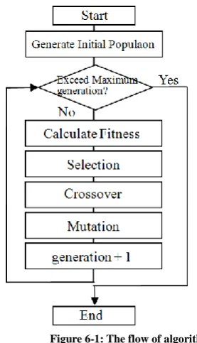
6.3 The flow of Algorithm

The flow of algorithm is exhibited in Figure 6-1.

Figure 6-1: The flow of algorithm

A. Initial Population

Generate M initial population. Here, M100 . Generate each individual so as to satisfy (22).

B. Calculation of Fitness

[image:5.612.39.298.479.559.2]

(6)

International Journal of Emerging Technology and Advanced Engineering

[image:6.612.68.269.146.510.2]

12

Figure 6-2:The flow of calculation of fitness

Scaling[15] is executed such that fitness becomes large when the variance of forecasting error becomes small. Fitness is defined as follows.

) , ( )

,

(₁₂ U_2 ₁₂

f

(30)

Where U is the maximum of 2(₁,₂)during the past Wgeneration. Here, W is set to be 5.

C. Selection

Selection is executed by the combination of the general elitist selection and the tournament selection. Elitism is executed until the number of new elites reaches the predetermined number. After that, tournament selection is executed and selected.

D. Crossover

Crossover is executed by the uniform crossover. Crossover rate is set as follows.

7 .

0 

c

P

(31)

E. Mutation

Mutation rate is set as follows.

05 .

0 

m

P

(32)

Mutation is executed to each bit at the probabilityP_m,

therefore all mutated bits in the population Mbecomes

14

 M

Pm .

VII. NUMERICAL EXAMPLE

7.1 Application to the manufacturer’s data of sanitary mat erials

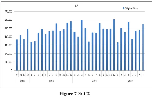
[image:6.612.322.573.384.700.2]

Manufacturer’s data of sanitary materials from September 2009 to August 2012are analyzed. Furthermore, GA results are compared with the calculation results of all considerable cases in order to confirm the effectiveness of GA approach. First of all, graphical charts of these time series data are exhibited in Figure 7-1 - 7-5.

Figure 7-1: A2

Figure 7-1: A2

(7)

International Journal of Emerging Technology and Advanced Engineering

[image:7.612.47.296.133.295.2]

13

Figure 7-3: C2

7.2 Execution Results

GA execution condition is exhibited in Table 7-1.

Table7-1 GA Execution Condition

GA Execution Condition

Population 100

Maximum Generation 50

Crossover rate 0.7

Mutation ratio 0.05

Scaling window size 5

The number of elites to retain 2

Tournament size 2

We made 10 times repetition and the maximum, average, minimum of the variance of forecasting error and the average of convergence generation are exhibited in Table 7-2 and 7-3.

Table7-2

GA execution results(Monthly ratio is not used)

The variance of forecasting error Average of convergence generation

Minimum Maximum Average

Product A2

10,789,82 5,203

12,498,19 4,197

10,977,67

2,566 14.0

Product B2

35,920,19 4,826

42,582,41 5,643

36,552,83

2,210 13.0

Product C2

13,783,38 6,901

16,475,40 0,903

14,083,28

6,823 9.0

Table7-3

GA execution results (Monthly ratio is used)

The variance of forecasting error Average of convergence generation Minimum Maximum Average

Product A2

8,938,904, 153

10,633,00 2,350

9,047,03

0,143 10.0

Product B2

14,891,21 9,928

21,900,93 6,794

15,242,9

78,448 14.0

Product C2

4,823,072, 577

8,009,433, 975

5,082,15

3,349 20.0

In all cases, the variance of forecasting error for the case monthly ratio is used is smaller than the case monthly ratio is not used.

The minimum variance of forecasting error of GA coincides with those of the calculation of all considerable cases and it shows the theoretical solution. Although it is a rather simple problem for GA, we can confirm the effectiveness of GA approach. Further study for complex problems should be examined hereafter.

Figure7-6: A2 (Monthly ratio is not used)

Figure7-6:A2(Monthly ratio is not used)

Figure7-7: A2 (Monthly ratio is used)

(8)

International Journal of Emerging Technology and Advanced Engineering

14 Figure7-8: B2 (Monthly ratio is not used)

Figure7-8:B2(Monthly ratio is not used)

Figure7-9:B2(Monthly ratio is used)

Figure7-10:C2(Monthly ratio is not used)

Figure7-11:C2(Monthly ratio is used)

Next, optimal weights and their genes are exhibited in Table 7-4, 7-5

Table7-4

Optimal weights and their genes (Monthly ratio is not used)

Data

1



₂



3

position of the bit

13 12 11 10 9 8 7 6 5 4 3 2 1 0

Product A2 0.46 0.54 0 0 1 1 1 0 1 1 1 0 0 0 1 0 1

Product B2 1.00 0 0 1 1 1 1 1 1 1 0 0 0 0 0 0 0

(9)

International Journal of Emerging Technology and Advanced Engineering

15

Table7-5

Optimal weights and their genes (Monthly ratio is used)

Data

1



2



3

position of the bit

13 12 11 10 9 8 7 6 5 4 3 2 1 0

Product A2 0.69 0.31 0 1 0 1 1 0 0 0 0 1 0 0 1 1 1

Product B2 1.00 0 0 1 1 1 1 1 1 1 0 0 0 0 0 0 0

Product C2 0.21 0.79 0 0 0 1 1 0 1 1 1 1 0 0 1 0 0

In the case monthly ratio is used, the 1st+2nd order f unction model is best in Product A2 and Product C2,while Product B2 has selected the linear model as thebest one.

Parameter estimation results for the trend of equation (21) using least square method are exhibited in Table 7-6 for the case of 1st to 24th data.

Table7-6

Parameter estimation results for the trend of equation (21)

Data

1

a

b

₁

a

₂

b

₂

c

₂

a

3

b

3

c

3

d

3

Product A2 738.11782

6 634859.15

-496.9376

6 13161.559

581024.23 9

-29.38027

3 604.82257

1917.7289

3 606805

Product B2 2173.3321

7 612274.26

-458.3867

4 13633.001

562615.70 1

125.01876

8 -5146.591

61477.683

2 452911.73

Product C2 4559.1178

3 403455.9

-538.0480

2 18010.318

345167.36 7

-6.192786

8 -305.8185

15640.338 7

350601.53 75

Trend curves are exhibited in Figure 7-16 - 7-20.

Figure7-16: Trend of A2

(10)

International Journal of Emerging Technology and Advanced Engineering

16

Figure7-18: Trend of C2

Calculation results of Monthly ratio for 1st to 24th data are exhibited in Table 7-7.

Table7-7:

Parameter Estimation result of Monthly ratio

Date. 1 2 3 4 5 6 7 8 9 10 11 12

Product A2 0.906 1.113 0.891 1.201 0.903 0.871 1.088 1.162 0.859 1.066 0.972 0.967

Product B2 1.029 0.996 0.834 1.288 0.665 0.907 1.040 1.353 0.764 1.083 1.052 0.987

Product C2 0.976 1.041 1.046 1.186 0.867 0.809 1.108 1.052 0.822 0.957 0.965 1.170

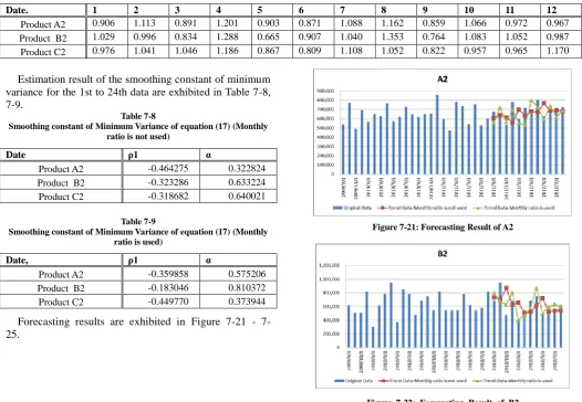
Estimation result of the smoothing constant of minimum variance for the 1st to 24th data are exhibited in Table 7-8, 7-9.

Table 7-8

Smoothing constant of Minimum Variance of equation (17) (Monthly ratio is not used)

Date ρ1 α

Product A2 -0.464275 0.322824

Product B2 -0.323286 0.633224

Product C2 -0.318682 0.640021

Table 7-9

Smoothing constant of Minimum Variance of equation (17) (Monthly ratio is used)

Date, ρ1 α

Product A2 -0.359858 0.575206

Product B2 -0.183046 0.810372

Product C2 -0.449770 0.373944

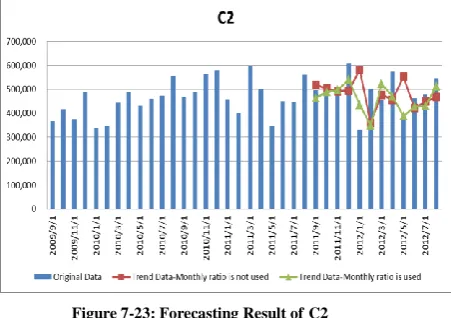
Forecasting results are exhibited in Figure 21 - 7-25.

Figure 7-21: Forecasting Result of A2

[image:10.612.43.570.313.677.2]

(11)

International Journal of Emerging Technology and Advanced Engineering

[image:11.612.68.294.143.302.2]

17

Figure 7-23: Forecasting Result ofC2

7.3 Remarks

In all cases, the variance of forecasting error for the case monthly ratio is used is smaller than the case monthly ratio is not used. In the case monthly ratio is used, the 1st+2nd order function model is best in Product A2 and Product C2, while Product B2 has selected the linear model as the best one.

The minimum variance of forecasting error of GA coincides with those of the calculation of all considerable cases and it shows the theoretical solution. Although it is a rather simple problem for GA, we can confirm the effectiveness of GA approach. Further study for complex problems should be examined hereafter.

VIII. CONCLUSION

Focusing on the idea that the equation of exponential smoothing method(ESM) was equivalent to (1,1) order ARMA model equation, a new method of estimation of smoothing constant in exponential smoothing method was proposed before by us which satisfied minimum variance of forecasting error. Generally, smoothing constant was selected arbitrary. But in this paper, we utilized above stated theoretical solution. Firstly, we made estimation of ARMA model parameter and then estimated smoothing constants. Thus theoretical solution was derived in a simple way and it might be utilized in various fields.

Furthermore, combining the trend removal method with this method, we aimed to improve forecasting accuracy. An approach to this method was executed in the following method. Trend removal by a linear function was applied to the manufacturer’s data of sanitary materials. The combination of linear and non-linear function was also introduced in trend removal.

Genetic Algorithm was utilized to search the optimal weight for the weighting parameters of linear and non-linear function. For the comparison, monthly trend was removed after that. Theoretical solution of smoothing constant of ESM was calculated for both of the monthly trend removing data and the non monthly trend removing data. Then forecasting was executed on these data. The new method shows that it is useful for the time series that has various trend characteristics. Various cases should be examined hereafter in order to confirm the effectiveness of this method.

REFERENCES

[1] Box Jenkins. (1994) Time Series Analysis Third Edition，Prentice Hall.

[2] R.G. Brown. (1963) Smoothing, Forecasting and Prediction of Discrete –Time Series, Prentice Hall.

[3] Hidekatsu Tokumaru et al. (1982) Analysis and Measurement – Theory and Application of Random data Handling, Baifukan Publishing.

[4] Kengo Kobayashi. (1992) Sales Forecasting for Budgeting, Chuokeizai-Sha Publishing.

[5] Peter R.Winters. (1984) Forecasting Sales by Exponentially Weighted Moving Averages, Management Science，Vol6，No.3, pp. 324-343.

[6] Katsuro Maeda. (1984) Smoothing Constant of Exponential Smoothing Method, Seikei University Report Faculty of Engineering, No.38, pp. 2477-2484.

[7] M.West and P.J.Harrison. (1989) Baysian Forecasting and Dynamic Models，Springer-Verlag，New York.

[8] Steinar Ekern. (1982) Adaptive Exponential Smoothing Revisited， Journal of the Operational Research Society, Vol．32 pp．775-782. [9] F.R.Johnston. (1993) Exponentially Weighted Moving Average

(EWMA) with Irregular Updating Periods, Journal of the Operational Research Society，Vol.44，No.7 pp．711-716. [10] Spyros Makridakis and Robeat L.Winkler. (1983) Averages of

Forecasts；Some Empirical Results，Management Science，Vol.29, No.9, pp. 987-996.

[11] Naohiro Ishii et al. (1991) Bilateral Exponential Smoothing of Time Series, Int.J.System Sci., Vol.12, No.8, pp. 997-988.

[12] Kazuhiro Takeyasu. (1996) System of Production, Sales and Distribution, Chuokeizai-Sha Publishing.

[13] Kazuhiro Takeyasu and Kazuko Nagao.(2008) Estimation of Smoothing Constant of Minimum Variance and its Application to Industrial Data, Industrial Engineering and Management Systems, vol.7, no. 1, pp. 44-50.

[14] Masatosi Sakawa. Masahiro Tanaka. (1995）Genetic Algorithm、Asakura Pulishing Co., Ltd.

[15] Hitoshi Iba.（2002）Genetic Algorithm、Igaku Publishing. [16] Daisuke Takeyasu and Kazuhiro Takeyasu.(2013) Estimation of