Estimating the Final Cost of Construction Project
Using Neural Networks: A Case of Yemen
Construction Projects
Asem Ali Ahmed Alshahethi1, K. L. Radhika2 1
Post Graduation Student, 2Associate Professor, Department of Civil Engineering, Osmania University, Hyderabad, India
Abstract: Cost is an important aspect to everyone, especially in the construction projects. For any project requires accurate cost diction in order to inspire the decision either forward or cancel the project. Moreover, predicting the cost plays a key role in the successful completion of the construction projects. Due the lack in information, details, drawings and many important factors that affecting in estimation the cost during planning phase, the project will be at risk. Therefore, the cost estimation plays a significant role in construction project decisions and represents the most important corner in iron triangle of construction management. In order to success the construction projects we need technique to estimate the cost with high degree of accuracy and less error. In the present investigation, the model built by applying both quantitative approach and qualitative approach to identify the factors (variables) as inputs of the model. 85 projects are used for developing, training and testing the ANNs model, the output of this model is the expected construction costs of the projects. To validate the model, 14 projects as sample have tested to predict the cost with high degree accuracy and acceptable error. Consumer Price Index, cost of construction materials, type of building, market conditions, structural system, site Area, type of slab, other Supplementary buildings, location of the Project, project Size, type of foundation, building closeness, and fluctuation in the Currency are the main factors affecting in construction buildings costs. These factors have been used as inputs in ANN model and all data is extracted from the historical projects, the model has been developed and trained for 70 projects and compared the actual cost with predicted cost. The model was validated throughout sample of projects. 13- 17- 1 model was the best between 15 models are developed, 6% is the mean absolute percentage error for model is tested. The results are clearly provided a good indicator for predicting the construction buildings costs in the future with high degree of accuracy.
Keywords: Cost Factors, Artificial Neural Network System, Feed Forward Network, Multilayer Perceptron, Back Propagation
Error, Developing the model.
I. INTRODUCTION
Fig. 1: Iron Triangle in Construction Management
II. LITERATUREREVIEW
Kumar Neeraj JHA2004 (1-6), Cost estimates of different accuracies are required by different agencies for different purposes in different stages of the project! The primary objective of an estimate is to enable one to know beforehand the cost of the work, though the actual cost is only known after the completion of the work from the accounts of the complete work. If the estimate is prepared carefully, there will not be much difference in the estimated cost and actual cost. For accurate estimate, the estimator should be experienced and fully acquainted with the method of construction. The estimate may be prepared approximately in a manner explained earlier or may be made in details, item-wise. In general, a choice of the method estimation to be used depends upon the nature of the project, the life- cycle phase, the purpose for which the estimate is required, the degree of accuracy desired and the estimating effort employed. AL-Zwainy 2012[4], Neuron computing architectures can be built into physical hardware (or neuron computer, or machine) or neuron software languages (or programs) that can think and act intelligently like human beings. Among various architectures and paradigms, the back-propagation network is one of the simplest and most practicable networks being used in performing higher level human tasks such as diagnosis, classification, decision-making, planning, and scheduling. The neural network based modeling process involves five main aspects: (1) data acquisition, analysis and problem representation; (2) architecture determination; (3) learning process determination; (4) training of the network; and (5) testing of the trained network for generalization evaluation, (Wu and Lim 1993).Ajibade Ayodeji Aibinu, et al. 2011(5) Pre-tender estimates are susceptible to inaccuracies (biases) because they are often prepared within a limited timeframe, and with limited information about project scope. Inaccurate estimation of project uncertainties is the underlying cause of project cost overruns in construction. Hashem AL-Tabatbi 1997(7), a neural network model to predict cost performance of construction project is presented, first knowledge representation formalism for cost performance prediction is developed, considering various direct cost elements, and second, the capability of networks, as mapping tools is explored to develop a relation between the construction environmental variables and the project cost performance.
Dr. Zeyad S. et al. 2014(9), A neural network was developed to predict the early stage cost of the buildings. A large number of data was collected from different structure for developing and training lf the ANN model. There are seven key parameters influencing the cost of buildings, the ANN model had one hidden layer with seven neurons, one neuron representing the early cost estimate of the buildings formed the output layer off the ANN model. Roxas, et al. 2014(10), The ANN approach provided good predicting ability despite the non-uniform distribution and incompleteness of the data set. Statistical analysis can be performed like considering the type of the building, weather low rise, mid-rise and high rise. Extensive manipulation of the data to be used the MATLAB program can be explored to improve the results. A. M. El- Kholy 2015 (12), the second model based on case based reasoning. Validation of the two models revealed that regression model has prediction capabilities higher than that of CBR model in predicting cost overrun percentage for construction projects. On the other hand, testing the case based reasoning model's effectiveness with respect to the weight assignment method for attributes revealed that best results are obtained when applying absolute standardized
III.METHODOLOGY
To develop the parameters cost estimation model by applying the artificial neural networks methodology is the essence of this research, which takes the building projects to predict the final cost of construction building projects. This study adopts upon the historical data to training this methodology, using the main factors affecting as inputs to provide historical data to make estimation cost for new projects. The necessary information and required projects data were collected to build the model of estimation construction cost of building projects.
Conceptual cost estimation, cost control, cost overrun, cost codes and cost management are reviewed to identify the main topics to be handled in this research. All types of artificial neural networks (ANNs), their structure, and applications are outlined. To achieve the objective of the research, development artificial neural networks model for construction projects cost. The research strategy can be classified into two types namely, quantitative approach and qualitative approach. The both types quantitative and qualitative approach are used to collect thee data of the projects and thee information about the factors which influencing in the construction building cost.
This research methodology consists from two stages:
A. Research Strategy
1) Theoretical study : It is involving review the cost estimation and (ANNs) technique from the references, thesis, journal papers, and books were published in project management field relating to the subject of research
2) Field work : It is involving the following steps:
3) Description and selection the factors that influencing the costs of building construction projects. 4) Pilot study involving interviews are used to modify and improve the draft questionnaire
5) Factors are identified and categorized in different groups before sending the final questionnaire to collect the respondents 6) A questionnaire survey methodology is employed to determine and rank these factors according to their levels of influence on
the cost of building construction project using SPSS program.
7) Developing of NN model to predict the cost of building construction projects using MATLAB SOFTWARE program. 8) Validation of the NN model.
B. Historical Data Collection
Based on thesis methodology and after determining the most important factors, data for training and testing the proposed artificial neural networks model were collected. These data were gathered from real life projects conducted from 2000 to 2017 in Yemen. This process was done using a data collection. (86) Construction buildings projects are collected from Yemen. All data required to construct the model have been collected from ministry of work in Yemen and the companies that executed these projects to compare the estimation value with actual cost.
IV.COST PREDICTION USING NEURAL NETWORKS
This chapter explains the incorporation of the previously identified cost factors into construction buildings. These factors that affecting in construction buildings costs are investigated to be as inputs in ANN model to predict the total cost of construction buildings in Yemen. As mentioned in chapter three, 85 projects are prepared and arranged for developing the ANN model. The data is deduced from 85 projects by Microsoft Excel to import it directly into MATLAP program as inputs and outputs.
First step in this chapter is designing the ANN model regarding on the data was collected and analyzed, thereafter, throughout the artificial neural networks technique is applied to prepare cost prediction model. Finally, three processes have done by MATLAB program namely, training, testing, and validating the best model with lees error and highest accuracy.
A. Design the ANN model
Designing ANN models are divided into five basics steps namely, (1) Collecting the data, (2) preprocessing data, (3) architecture the network, (4) training the model, and (5) testing the performance of model.
2015.
2) Data Pre-processing : After data collection, the variables were analyzed using mathematical and software methods such a Microsoft Excel and SPSS23 program, to select the main factors that affecting in construction buildings costs.The data preprocessing procedures are conducted to train the ANNs model more efficiently. These procedures are, (1) solve the problem of missing data from the projects, (2) normalize data, and (3) randomize data. The missing data is replaced by Assuming the value that is the nearest to reality such as, some projects the area of them is missing and not founded, regarding to the insulation layer of building surface in (m2) is taken as area value.
3) Architecture the Network: The neural network was built to consist of three parts, the input layer, hidden layers, and output layer. The weights are linked between these layers, all nodes enclosed by weights from inputs to hidden layer and also from hidden layer to output layer.
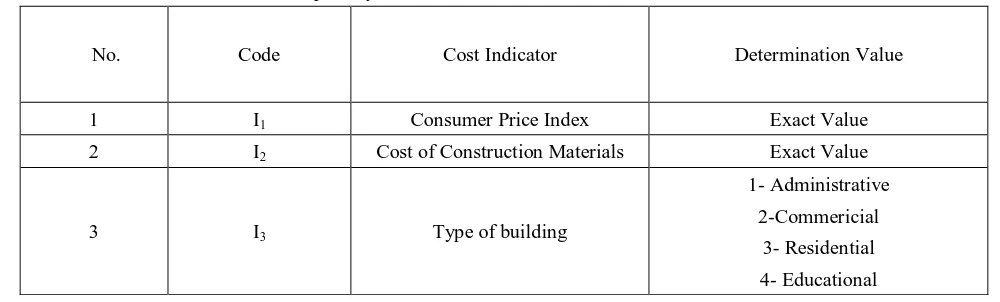
4) Input layer, the first one, enclosing 13 nodes, each node represents one of the selected cost indicators, as concluded in the previous chapter, each cost indicator will be determined by a value; for quantitative indicators, the exact value will be used, however, for qualitative indicators, a preselected value will be used as an indicator for each case, table 1 illustrates the cost indictors used in the input layer and the correspondent determination value for each cost indicator. Finally, all the data in this layer will be scaled from (-1) to (1).
5) Hidden Layer(s), the second ordered layer. In this layer(s), the number on nodes (hidden nodes) ware calculated by considering one guidance that the number of hidden nodes must be not less than half the summation of the number of nodes in the input and output layers (Hosny 2011). According to that guidance, the number of hidden nodes will be calculated according to equation 4.1.
Minimum hidden nodes
=∑( ) ...4.1
According to the previous guidance, 10 and above hidden nodes were used in this layer, also an activation function will be used to activate data derived into these hidden nodes. In the trial and error practices, another hidden layer will be added to a new model to be used in a deferent set of trials.
B. Activation Function
MATLAB provides built-in transfer functions which are used in this study; linear (purelin), Hyperbolic Tangent Sigmoid (logsig) and Logistic Sigmoid (tansig).
C. Feed-Forward Networks
Neurons in input layer only act as buffers for distributing the input signals xi (i=1, 2 …n) to neurons in the hidden layer. Each neuron j in the hidden layer sums up its input signals xi after weighting them with the strengths of the respective connections (wji) from the input layer and computes its output (yj) as a function f of the sum.
1
[
]
n
j ji i
i
y
f
w x
………...………..…………..……….………4.2
f can be a simple threshold function or a sigmoidal, hyperbolic tangent or radial basis function.
The output of neurons in the output layer is computed similarly. The back propagation algorithm, a gradient descent algorithm, is
the most commonly adopted MLP training algorithm. It gives the change Δwji the weight of a connection between neurons (i) and
(j) as follow steps:
Step 1: Initialize weight to small random values.
Step 2: While stopping condition is false, do steps 3-10. Step 3: For each training pair do steps 4-9.
Feed Forward
Step 5: Each hidden unit (zj, j = 1, …, p) sums its weighted inputs signals
1
n
inj oj i i ij
z
v
x v
……..……….…...………4.3
Applying activation function
Zj = f (z-inj) ……….………....4.4
And send this signal to all units in the above layer (output layer).
Step 6: Each output unit (yk, k = 1, …, m) sums its weighted input signals
1 p
ink ok j j jk
y
w
z w
……….……...4.5
and applies its activation function to calculate the output signals.
(
)
k ink
y
f y
………....………...………...4.6 D. Back Propagation of Error
The predictive models based upon ANN utilize back-propagation technique along with different training algorithms and methods available in MATLAB. In our research work these methods have been employed for prediction analysis of software estimation. Back-propagation utilizes techniques of supervised learning and presents a target with computed output in each of iteration for the tuning of the network, so that we keep moving toward the point of minimum error.
E. Back Propagation of Error Steps
Step 7:Each output unit (yk, k = 1, …, m) receives a target pattern corresponding to an input pattern, error information term is
calculated as
(
) (
)
k
t
ky
kf y
ink
……….……...4.7
Step 8: Each hidden unit (zj, j = 1, …, p) sums its delta inputs from units in the layer above
1 m
inj j jk
k
w
………..………...………..4.8 The error information term is calculated as(
)
k inj
f z
inj
………..………...……...…………...4.9 Step 9: Each output unit (Yk, k = 1, …, m) updates its bias and weight (j =0, …, p) the weight correction term is given by
jk k j
w
z
……….………..…………....4.10 And the bias correction in term is given by
ok k
w
………..………...4.11 Therefore, ( ) ( )jk new jk old jk
w
w
w
………...……..………..4.12
( ) ( )
ok new ok old ok
w
w
w
………..……..………...……….4.13 Each hidden unit (zj, j = 1, …, p) updates its bias and weights (i=0, …. n), the weight correction term
ij j i
v
x
The bias correction term oj j
v
………...………..……..……….4.15 Therefore, ( ) ( )ij new ij old ij
v
v
v
………..………..…..……...………….………..4.16
( ) ( )
oj new oj old oj
v
v
v
………..………..……….…4.17
Where the various parameters used in the training algorithm are as follows. X: input training data.
x= (x1 …. xn).
t= (t1………tn).
ᵟk = error at output unit yk
ᵟj = error at hidden unit zj
α= learning rate.
Voj= bias on hidden unit j.
F. Testing the Model
In order to evaluate the performance of the developed ANN models quantitatively and verify whether there is any underlying trend in performance of ANN models, statistical analysis involving the coefficient of determination (R2), the root mean square error (RMSE), and the mean bias error (MBE) were conducted. RMSE provides information on the short term performance which is a measure of the variation of predicated values around the measured data. The lower the RMSE, the more accurate is the estimation. MBE is an indication of the average deviation of the predicted values from the corresponding measured data and can provide information on long term performance of the models; the lower MBE the better is the long term model prediction. A positive MBE value indicates the amount of overestimation in the predicated construction buildings costs. The expressions for the aforementioned statistical parameters are:
1
1
(
)
n predicted actual iMSE
I
I
n
………..………..………4.17 2 11
(
)
n predicted actual iRMSE
I
I
n
………..……….……….………4.18
Where Ip, i denotes the predicted construction buildings costs in (R.Y.). Ii denotes the measured construction buildings costs in (R.Y.), and n denotes the number of observations.
IV. RESULTS AND DISUCSSION
A. Programming The Nn Model
MATLAB (2015a) is used to write script files for developing ANN models and performance functions for calculating the error statistics as R2, RMSE and MSE. It allows the designer to prepare easy matrix manipulation, plotting of functions and data, implementation of algorithms and also provides comprehensive support and enables the user to design and manage the neural networks in a very simple way.
The MLP program starts by reading data from excel file (training data and testing data). “xlsread” function is used to read the data from excel sheets.
Data Target= xlsread ('target data.xlsx');
Data Test = xlsread ('testing data.xlsx');
Training data samples are 70 projects prepared to train the model (training samples).
MATLAB helps devise the MLP model by using a feed –forward back propagation network, number of hidden layers, the neurons in each layer, transfer function in each layer, the training function, the weight/ bias, learning function and the performance function have been done throughout designing the NN networks.
My network = newff(input, target, i, tf);Where tf denotes to transfer function.
i denotes to the number of neurons in hidden layer. MyNetwork. trainFcn = Rb;
MyNetwork.trainparam.min_grad = 0.00000001;
MyNetwork.trainParam.epochs = 1000;
MyNetwork.trainParam.lr = 0.01;
MyNetwork.trainParam.max_fail =1000; Where
“trainFcn”: defines the function used to train the network. It can be set to the name of any training function (LRb 'trainRb%Bayesan Regularization back-propagation).
“trainparam.min_grad”: denotes the minimum performance gradient. “trainParam.epochs”: denotes the maximum number of epochs to train.
“trainParam.lr”: denotes the learning rate.
“trainParam.max_fail”: denotes the maximum validation failures.The MLP network is trained using “trainFcn” train function.
MyNetwork = train(MyNetwork,input,target);The MLP network is tested using “simFcn” testing function. MyNetwork = train(MyNetwork, test);
B. Developing ANN Model Using MATLAB
MATLAB (2015a) is used to write script files for developing ANN models and performance functions for calculating the error statistics as R2, RMSE and MSE. It allows the designer to prepare easy matrix manipulation, plotting of functions and data, implementation of algorithms and also provides comprehensive support and enables the user to design and manage the neural networks in a very simple way. Table 1 is shown the input layer and the determination value for each cost indicator (inputs data).
When the training is complete, the network performance should be checked. Therefore, unseen data (testing) will be exposed to the network. Figure.2 and Figure.3 show, respectively, screen captions of the MLP training windows obtained using the “nntraintool”
[image:8.612.54.554.589.740.2]GUI toolbox in MATLAB.
Table 1: The Input Layer and the Determination Value for Each Cost Indicator
No. Code Cost Indicator Determination Value
1 I1 Consumer Price Index Exact Value
2 I2 Cost of Construction Materials Exact Value
3 I3 Type of building
1- Administrative
2-Commericial
4 I4 Market Conditions
1- International Market 2- Regional Market
5 I5 Structural System
1- Concrete
2- Steel
3- Mix
6 I6 Site Area Exact Value
7 I7 Type of Slab
1-Solid Slab
2- Hollow Block 3- Flat Slab
8 I8 Other Supplementary Buildings Exact Value
9 I9 Location of the Project
1- Inside Sana’a
2- Outside (Mountain Area) 3- Outside (Coastal Area) 4- Outside (Desert Area)
10 I10 Project Size
1- Huge 2- Medium 3- Small
11 I11 Type of Foundation
1- Isolated Foundation 2- Combined Foundation 3- Strip Foundation 4- Raft
5-Pile
12 I12 Building Closeness
1- Attached 2- Semi- Attached 3- Separated
13 I13 Fluctuation in the Currency Exact Value
Fig.3: Plot Regression Windows
V. RESULTS AND DISSECTION
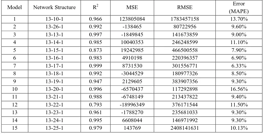
This section presents the best achieved results for MLP models. In table 2 is shown the computed values of R2, MSE, and RMSE for (15) developed ANN models. The network structure is involved three layers and denoted by three numbers, first number indicates the number of neurons in the input layer, second number indicates of the number of neurons in the hidden layer, and third number refers of the neuron in the output layer. (70) Samples are used for training each model, (14) samples are tested of each model. (15) Models are developed.
Table 2: Statistical error parameters of developed MLP models for different network structures
Model Network Structure R2 MSE RMSE Error
(MAPE)
1 13-10-1 0.966 123805084 1783457158 13.70%
2 13-26-1 0.992 -138465 80722956 9.60%
3 13-13-1 0.997 -1849845 141673859 9.00%
4 13-14-1 0.985 10040353 246248599 11.10%
5 13-15-1 0.873 19242985 466500558 7.90%
6 13-16-1 0.983 4910198 220396357 6.90%
7 13-17-1 0.999 8731530 301556771 6.33%
8 13-18-1 0.992 -3044529 180977326 8.50%
9 13-19-1 0.947 2129605 383907356 9.30%
10 13-20-1 0.996 -6570437 117292898 16.56%
11 13-21-1 0.988 -6748149 213437822 9.40%
12 13-22-1 0.793 -18996349 376171544 11.50%
13 13-23-1 0.961 -1788270 235681033 9.30%
14 13-24-1 0.995 6608044 146971992 9.30%
15 13-25-1 0.979 143769 2408141631 10.13%
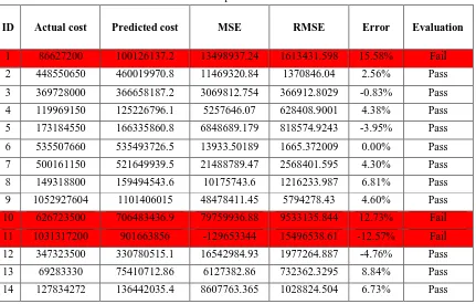
[image:10.612.75.536.493.729.2]Table 3: Statistical error parameters of model 13-17-1
ID Actual cost Predicted cost MSE RMSE Error Evaluation
1 86627200 100126137.2 13498937.24 1613431.598 15.58% Fail
2 448550650 460019970.8 11469320.84 1370846.04 2.56% Pass
3 369728000 366658187.2 3069812.754 366912.8029 -0.83% Pass
4 119969150 125226796.1 5257646.07 628408.9001 4.38% Pass
5 173184550 166335860.8 6848689.179 818574.9243 -3.95% Pass
6 535507660 535493726.5 13933.50189 1665.372009 0.00% Pass
7 500161150 521649939.5 21488789.47 2568401.595 4.30% Pass
8 149318800 159494543.6 10175743.6 1216233.987 6.81% Pass
9 1052927604 1101406015 48478411.45 5794278.43 4.60% Pass
10 626723500 706483436.9 79759936.88 9533135.844 12.73% Fail
11 1031317200 901663856 -129653344 15496538.61 -12.57% Fail
12 347323500 330780515.1 16542984.93 1977264.887 -4.76% Pass
13 69283330 75410712.86 6127382.86 732362.3295 8.84% Pass
14 127834272 136442035.4 8607763.365 1028824.504 6.73% Pass
A. Results and Discussion
From 15 models, one model is selected (model 7) to be the best model among all models is investigated. Network structure of model 10 is 13-17-1 and the statistical parameters are the lowest.
Seventh model, sixth model, fifth model, and eighth model have the better accuracy for predicting the construction buildings costs. The coefficient of determination R2 is 0.998, 0.997, 0.996 and 0.992 for the models 11, 13, 10 and 8 respectively.
[image:11.612.94.525.86.361.2]Model 7 has the lowest error is 6.33% and the model 10 has the highest error is 16.56%.
Table 3 is shown the results of the model 13-17-1 using ANN technique. The validation was done through 14 projects are tested, 11 projects passed and the error is accepted and 3 projects failed due missing data. MAPE of this model is calculated as 6% and this value is accepted by low of government (The value to be accepted must be + or – 10% in bidding award). 17 neurons are used in the hidden layer in this model to predict the construction buildings costs; therefore, %Error for these projects in the 13-17-1 model is accurate and reliable enough to be used as a predicting tool at conceptual stage
VI. CONCLUSION
In this study investigation, two stages were carried out to achieve the objectives. Data collection and analysis, and developing ANN model have been done. This study is deduced in few points as following:
Fifteen (15) NNs models were built to predict the cost of the project by using neural network Tool Box software by MATLAB program Through five attributes were taken as predictor variables namely; collect data, preprocessing data, architecture the network, training the model, and testing the model using excel sheet and MATLAP. RMSE, MSE, MAPE, and R2 were calculated and compared for all 15 models to show the best model. It is observed the error from Bayesan Regularization- back propagation shown the best convergence towards minimum error compared to other algorithms. Among those models is 13- 17- 1 model as its percentage of error is 6% which is the least mean absolute percentage error and its coefficient of determination is 0.9998 for models that have already been tested.
The findings clearly provide a good indicator for predicting the construction costs in the future with high degree of accuracy by using artificial neural network method.
A. Recommendations for Further Study
increased validity to the findings of this thesis: For cost estimation, it is suggested to study all factors separately or as groups and develop the best model, the data collected are not sufficient to cover all government buildings, thus we have to collect more than and add them to the model to improve the error and the missing data must be collected. The model should be augmented to take into consideration the other different types of construction projects. For example: the medical, commercial and other administrative construction projects. The model should be applied to predict the duration, productivity, risk analysis, and claims in construction projects.
REFERENCES [1] Kumar Neeraj JAH 2012. Text Book, “Construction Project Management’’
[2] Wayne j. Del Pico Text book 2012. “Estimating Building Costs for the Residential & Light Commercial Construction Professional”.
[3] Eng. Omar M. Shehatto. June 2013.” Cost estimation for building construction projects in Gaza Strip using Artificial Neural Network (ANN)”. Master thesis in construction management, The Islamic University of Gaza Stri
[4] Faiq Mohammed Sarhan Al-Zwainy2012, Development of The Construction Productivity Estimation Model Using Artificial Neural Network for Finishing Works for Floors with Marble, Baghdad, Iraq
[5] Dr. Ajibade Ayodeji Aibinu. “Use of Artificial Intelligence to Predict the Accuracy of Pretender Building Cost Estimate” Management and Innovation for a Sustainable Built Environment ISBN 20 – 23 June 2011, Amsterdam, the Netherlan
[6] K.C. Iyer, K.N. Jha. ‘’Factors Affecting Cost Performance: Evidence from Indian Construction Projects’’ International Journal of Project Management 23 (2005) 283- 295
[7] Hashem AL-Tabatbi 1997. ‘’Prediction of Cost Performance in Construction Projects Using Artificial Neural Networks’’, Kuwait.
[8] Alqahtani and Andrew Whyte, 2013. ’’Artificial Neural Networks Incorporating Cost Significant Items towards Enhancing Estimation for (life-cycle) Costing of Construction Projects’’. Australia
[9] Dr. Zeyad S. M. Khaled, 2014. ’’Modeling Final Costs of Iraqi Public School Projects Using Neural Networks’’, International Journal of Civil Engineering and Technology (IJCIET).
[10] Roxas, Cheryl Lyne, 2014. ’’Artificial Neural Network Approach to Structural Cost Estimation of Building Projects’’, Philippine
[11] Changiz Ahbab, 2012. ’’An Investigation on Time and Cost Overrun in Construction Projects’
[12] A. M. El-Kholy 2015, Predicting Cost Overrun in Construction Projects. International Journal of Construction Engineering and Management 2015, 4(4): 95-105 DOI: 10.5923/j.ijcem.20150404.0
[13] Hegazy, T. & Ayed, A., 1998. Neural Network Model for Parametric Cost Estimation of Highway Projects. Journal of Construction Engineering and Management, pp. 210-218.
[14] Hegazy, T., Moselhi & O., P. F. &., 1994. Developing Practical Neural Network Applications Using Back- Propagation. Microcompurers in Civil Engineering, Volume 9, pp. 145- 159
[15] Hegazy, T. & Moselhi, O., 1995. Elements of Cost Estimation: A Survey in Canada and the United States. Cost Engineering, 37(5), pp. 27-3
[16] Kim, G.-H., An, S.-H. & Kang, K.-I., 2004. Comparison of construction cost estimating models based on regression analysis, neural networks, and case-based reasoning. Building and Environment, February, Volume 39, p. 1235 – 124
[17] Adeli, H. & Wu, M. Y., 1998. Regularization neural network for construction cost estimation. Journal of Construction Engineering and Management-Asce, 124(1), pp. 18-2
[18] Bouabaz, M. & Hamami, M., 2008. A Cost Estimation Model for Repair Bridges Based On Artificial Neural Network. American Journal of Applied Sciences, 5(4), Pp. 334-33
[19] Al-Najjar, H., 2005. Prediction of Ultimate Shear Strength of Reinforced Concrete Deep Beams Using Artificial Neural Networks, Gaza Strip. Master Thesis in Construction Management, The Islamic University of Gaza Stri
[20] Principe, J. et al., 2010. NeuroSolution Help, s.l.: NeuroDimension, Inc