R E S E A R C H
Open Access
Preconditioning methods for solving a
general split feasibility problem
Peiyuan Wang
1,2*, Haiyun Zhou
2,3and Yu Zhou
2Dedicated to Professor Shih-sen Chang on the occasion of his 80th birthday.
*Correspondence:
[email protected] 1The Second Training Base, Naval
Aviation Institution, Huludao, 125001, China
2Department of Mathematics,
Shijiazhuang Mechanical Engineering College, Shijiazhuang, 050003, China
Full list of author information is available at the end of the article
Abstract
We introduce and study a new general split feasibility problem (GSFP) in a Hilbert space. This problem generalizes the split feasibility problem (SFP). The GSFP extends the SFP with a nonlinear continuous operator. We apply the preconditioning methods to increase the efficiency of the CQ algorithm, two general preconditioning CQ algorithms for solving the GSFP are presented. We also propose a new inexact method to approximate the preconditioner. The convergence theorems are established under the projections with respect to special norms. Some numerical results illustrate the efficiency of the proposed methods.
MSC: 46E20; 47J20; 47J25; 47L50
Keywords: general split feasibility problem; general variational inequality; preconditioning method; projection method
1 Introduction
As preconditioning methods can improve the condition number of the ill-posed system matrix, the convergence rate of the iterative algorithm can also be improved []. In [, ], a preconditioning method is applied to modify the projected Landweber algorithm for solving a linear feasibility problem (LFP). The modified algorithm is
xn+=PC
xn–τDA∗(Axn–b)
, n≥,
whereτ ∈(, /DA∗A),A:X→Y is a linear and continuous operator, · means -norm,XandY are Hilbert spaces andb∈Y is the datum of the problem, corrupted by noise or experimental errors.
While under the nonlinear conditions, Auslender and Dafermos [, ] proposed an al-gorithm to solve variational inequalities (VI),
xn+=PS
xn–τnG–F(xn)
, n≥, (.)
wherePSis the projection operator ontoSwith respect to the norm · G. Bertsekas and
Gafni [] and Marcotte and Wu [] improved it with variable symmetric positive defined matricesGn, Fukushima [] modified it by a relaxed projection method with half-space;
then in [], Yang established the convergence of Auslender’s algorithm under the weak co-coercivity ofF.
Further, the general variational inequality problem (GVIP) has been investigated by many authors (see [–]). It is to findu∗∈Rnsuch thatg(u∗)∈Kand
Fu∗,g(u) –gu∗≥, g(u)∈K,
whereKis a nonempty closed convex set inRn,F,g:Rn→Rnare nonlinear operators. In
[], Santos and Scheimberg extended and applied (.) to solve the GVI.
However, a general split feasibility problem (GSFP) equals to a GVI, and precondition-ing methods for solvprecondition-ing the GSFP have not been studied. By introducprecondition-ing a convex mini-mization problem, the split feasibility problem (SFP) is equivalent to a variational inequal-ity problem (VIP), which involves a Lipschitz continuous and inversely strong monotone (ism) operator, see [–]. Similarly, by the same way, in this paper we introduce that a new GSFP equals to a GVI involving a Lipschitz continuous and co-coercive operator [, –].
Otherwise, Mohammad and Abdul [] considered a general split feasibility in infinite-dimensional real Hilbert spaces. It is to findx∗such that
x∗∈ ∞
i=
Ci, Ax∗∈
∞
j=
Qj,
where A:H→H is a bounded linear operator, {Ci}∞i= and{Qj}∞j= are the families of
nonempty closed convex subsets ofHandH, respectively.
LetCandQbe nonempty closed convex subsets in real Hilbert spacesHandH,
re-spectively. We consider a general split feasibility problem which is different from the one in []. Our GSFP is to find
x∗∈H,g
x∗∈Csuch thatAgx∗∈Q, (.)
whereA:H→His a bounded linear operator andg:H→Cis a continuous operator.
We see that the SFP in [] and the GSFP in [] are particular cases of GSFP (.). It has applications in many special fields such as signal decryption, demodulating the digital sig-nal and noise processing,etc.In order to solve GSFP (.), two preconditioning algorithms are developed in this paper following the iterative scheme
g(xn+) =PC
g(xn) –γDA∗(I–PQ)Ag(xn)
, n≥,
where the two general constraintsCandQdeal with projections with respect to the norms corresponding to some symmetric positive definite matrices. Define the solution set of (.) ={x∗ ∈H|Ag(x∗)∈Q}, as is nonempty, and by virtue of the relatedG
-co-coercive operator, we can establish the convergence of the proposed algorithms.
2 Preliminaries
In what follows, we state some concepts and propositions.
The SFP is to find a pointx∗∈Csuch thatAx∗∈Q, whereA:H→His a bounded
linear operator [].
LetGbe a symmetric positive definite matrix, and setD=G–. Then the norm · G
is defined byxG=x,Gx for∀x∈H. We denote byPCthe projection operator ontoC
with respect to the norm · G[],i.e.,
PC(x) =arg min
y∈C x–yG
.
Letλminandλmaxbe the minimum and the largest eigenvalues ofG, respectively. Then
for the -norm · [, ], we have
λminx≤ xG≤λmaxx, ∀x∈H. (.)
Proposition .[, ] Let C be a nonempty closed convex subset in H,for∀x,y∈H and
∀z∈C,the G-projection operator onto C has the following properties:
(i) G(x–PCx),z–PC(x) ≤;
(ii) x±yG=xG ±x,Gy +yG;
(iii) PC(x) –PC(y)G≤ x–yG –(PC(x) –x) – (PC(y) –y)G.
LetD˜ be a symmetric positive definite matrix, andATD˜ =DAT. Then the norm ·
˜
D
is defined byyD˜ =y,Dy˜ for∀y∈H. We denote byPQthe projection operator ontoQ
with respect to the norm · D˜. According to the SFP, when GSFP (.) has no solution (refer to [, , ]), we can define
fg(x) =
(I–PQ)Ag(x)
and
f˜g D(x) =
Ag(x) –PQAg(x)
˜
D= ˜
DAg(x) –PQAg(x)
,Ag(x) –PQAg(x)
,
f˜g
D(x) is also convex and continuously differentiable inH. Its gradient operator is
∇fDg(x) =DAT(I–P Q)Ag(x).
AsD=I, we define
∇fg(x) =AT(I–PQ)Ag(x),
∇fg(x) is also Lipschitz continuous.
Proposition . If we consider the constrained minimization problem
min f˜g
D(x)|x∈Hs.t. g(x)∈C
its stationary point x∗∈Hsatisfies ⎧
⎨ ⎩
x∗∈H,g(x∗)∈C such that
∇fDg(x∗),g(x) –g(x∗) ≥, ∀g(x)∈C,
which is a general variational inequality involving a Lipschitz continuous and G-co-coercive operator.
Proof For∀x,y∈H, from (.) and Lemma . in [], we have
∇fDg(x) –∇fDg(y)G ≤λmax(G)∇fDg(x) –∇f g D(y)
≤ λmax(D) λmin(D)
∇fg(x) –∇fg(y)
≤ λmax(D) λmin(D)
Lg(x) –g(y)
≤ λmax(D) λmin(D)
Lg(x) –g(y)G,
whereLis the largest eigenvalue ofATA; therefore, the operator∇fg
Dis Lipschitz
contin-uous,
∇fDg(x) –∇fDg(y),g(x) –g(y)
≥λmin(D)
∇fg(x) –∇fg(y),g(x) –g(y)
≥λmin(D)
L ∇fg(x) –∇fg(y)
≥ λmin(D)
L·λmax(D)
∇fg(x) –∇fg(y) D
= λmin(D) L·λmax(D)
D∇fg(x) –∇fg(y)
,GD∇fg(x) –∇fg(y)
= λmin(D) L·λmax(D)
∇fDg(x) –∇fDg(y)G.
Thus, the operator∇fDgis co-coercive.
3 Main results
In this section, we propose several modified CQ algorithms with preconditioning tech-niques and prove the convergence.
3.1 General preconditioning CQ algorithm
In this part, we have our first algorithm with fixed stepsize and preconditioner to solve GSFP (.). The algorithm is as follows.
Algorithm . Choose∀x∈Hsuch thatg(x)∈C, and letxn∈Hsuch thatg(xn)∈C,
then we calculatexn+such that
g(xn+) =PC
g(xn) –γ∇fDg(xn)
, n≥, (.)
whereγ ∈(,L·L
D),LandLDare the largest eigenvalues ofA
Now we establish the weak convergence of Algorithm ..
Theorem . Suppose that the operators g:H→C and g–:C→Hare continuous.If =∅,then the sequence{xn}generated by Algorithm.converges to the solution of GSFP
(.).
Proof Firstly, for∀x∗∈, we have
gx∗=PC
gx∗–γ∇fDgx∗.
From (.), (iii), (ii) and the definition of ism, we have
g(xn+) –g
x∗G
=PC
g(xn) –γ∇fDg(xn)
–PC
gx∗–γ∇fDgx∗G
≤g(xn) –g
x∗–γ∇fDg(xn) –∇fDg
x∗G
≤g(xn) –g
x∗G– γg(xn) –g
x∗,∇fg(xn) –∇fg
x∗
+γ∇fDg(xn) –∇fDg
x∗,∇fg(xn) –∇fg
x∗
≤g(xn) –g
x∗G–
γ
L –γ
L D
∇fg(xn) –∇fg
x∗, (.)
asLγ –γLD> , which implies that the sequence{g(xn) –g(x∗)G}n∈Nis monotonically
decreasing, then we can obtain that the sequence{g(xn) –g(x∗)G}n∈Nis also convergent, especially, the sequence{g(xn)}n∈Nis bounded. Consequently, we get from (.)
lim
n→∞∇fg(xn) –∇fg
x∗= lim
n→∞∇fg(xn)= . (.)
Moreover, for eachg(xn)∈C, from (iii) and (.), we have g(xn+) –g(xn)G≤γ∇fD(xn)G
≤γLD∇fg(xn)G≤γLD
λmax(G)∇fg(xn).
Then by virtue of (.) we have
lim
n→∞g(xn+) –g(xn)G= . (.)
Hence, there exists a subsequence{g(xj)}j∈Nof{g(xn)}n∈Nsuch that
lim
j→∞
g(xj+) –g(xj)G= .
Thus,{g(xj)}j∈N is also bounded.
sequence{g(xn)}n∈N; for the subsequence{g(xj)}j∈N, we have{g(xj)}j∈N→g(x¯) asj→ ∞.
After that, from (.) we obtain
lim
j→∞
∇fg(xnj)=∇fg(x¯)=A
TAg(x¯) –ATP
QAg(x¯)= ,
that is,Ag(x¯)∈Q.
We usex¯in place ofx∗in (.) and obtain that{g(xn) –g(x¯)G}is convergent. Because
its subsequence{g(xnj) –g(x¯)G} →, then we get that{g(xn)}n∈N converges tog(x¯) as j→ ∞. As well asg–is continuous, we finally have
lim
n→∞xn=x¯∈.
Therefore,x¯is a solution of GSFP (.).
From Algorithm . and Theorem . we can deduce the following results easily.
Corollary . If g=I,then GSFP(.)reduces to SFP, Algorithm.also reduces to a preconditioning CQ(PCQ)algorithm for∀x∈H:
xn+=PC
xn–γ∇fD(xn)
, n≥, (.)
whereγ ∈(,L·L
D),L and LDare the largest eigenvalues of A
TA and D,respectively.P Cand PQare still the projection operators onto C and Q with respect to the norm · Dand · D˜, respectively.
Corollary . If g=I,D=I,D˜ =I,then GSFP reduces to SFP,then Algorithm.reduces to the CQ algorithm proposed in[].
Corollary . If g=I,D˜ =I,PCand PQare the projections onto C and Q with respect to the norm · ,set F(xn) =DAT(I–PQ)ADxn, (.)transforms into the algorithm in[]
xn+=PC
xn–γF(xn)
, n≥,
whereγ ∈(,L),L=DAT.Then the GSFP reduces to the extended split feasibility
prob-lem(ESFP)in[].
3.2 An algorithm with variable projection metric
The algorithms above can speed the convergence of CQ algorithm, but the stepsize and preconditioner are fixed. In this subsection, we extend the results in [] and construct an iterative scheme with variable stepsize and preconditioner Dnfrom one iteration to
the next. As a key role,Dnwill change arbitrarily or following some rules to achieve the
convergence progress and better results.
LetDnandD˜nbe two symmetric positive definite matrices forn= , , , . . . . Denote
Algorithm . Choose∀x∈Hsuch thatg(x)∈C, and letxn∈Hsuch thatg(xn)∈C;
for∀Dn∈χ, we computexn+such that
g(xn+) =PC
g(xn) –γnDn∇fg(xn)
, n≥, (.)
whereγn∈(,L·MD),Lis the largest eigenvalue ofATA,MDis the minimum value of all
the largest eigenvalue valuesLDnto matricesDn.
Remark . Definedn=g(xn+) –g(xn)Gn, then for the next iteration,Dn+is either
cho-sen arbitrarily fromχor equivalent toDn. It is conditional on whetherdnhas decreased
or not. More particularly, we define a scalard¯nwith initial valued¯=∞. Having chosen a
scalarα∈(, ) at thenth iteration, thend¯n+is calculated by
¯
dn+= ⎧ ⎨ ⎩
αd¯n, ifdn≤ ¯dn;
¯
dn, ifdn>d¯n,
then we select
Dn+= ⎧ ⎨ ⎩
∀D∈χ, ifd¯n+<d¯n; Dn, ifd¯n+=d¯n.
Theorem . If=∅,then the sequence{xn}generated by Algorithm.converges to the solution of GSFP(.).
Proof To obtain variableDnat each iteration and keep the convergence of Algorithm ., dnmust be a descending behavior forn= , , , . . . . We first show that
lim
n→∞
dn= . (.)
Indeed if (.) is not true, we havelimn→∞dn> , thenDnmust have changed a finite
number of times, we set that this number isκ∈N. Therefore, letx∗∈be a solution of GSFP, refer to (.) and forn>κ, we have
g(xn+) –g
x∗G
κ ≤g(xn) –g
x∗G κ
–
γκ
L –γ
κLDκ
∇fg(xn) –∇fg
x∗,
asMD=min{LDn |n= , , . . .κ},
γκ
L –γ
κLDκ > . Then, following the proof of Theo-rem ., we also get
lim
n→∞∇fg(xn)= (.)
and
lim
n→∞dn=nlim→∞g(xn+) –g(xn)Gκ = . (.)
By using (.) and (iii), for thenth iteration, we have
dn=g(xn+) –g(xn) Gn
≥
g(xn) –PC
g(xn)Gn–g(xn+) –PC
g(xn)Gn
=
g(xn) –PC
g(xn) Gn–PC
g(xn) –γnDn∇fg(xn)
–PC
g(xn) Gn
≥
g(xn) –PC
g(xn)Gn–γnLDn∇fg(xn)
Gn,
whereγnLDn> . Then from (.) and (.) we know that
lim
n→∞∇fg(xn)Gn=nlim→∞A
T(I–P
Q)Ag(xn)Gn= ,
soAg(xn)∈Q. By virtue of (.), we also have
lim
n
g(xn) –PC
g(xn)= .
This means that at least a subsequence of{g(xn)}n∈N converges to a solution ofg(x¯)∈. Similar to the argumentation of accumulation in the proof of Theorem ., we know that
{xn}converges to a solution of GSFP.
3.3 Some methods for execution
In Algorithms . and ., there still exists difficulty to implement the projectionsPCand PQwith respect to the defined norms, especially whenCandQare general closed convex
sets. According to the relaxed method in [, , ], we consider the above algorithm in which the closed convex subsetsCandQare the following particular formula:
C= g(x)∈H|c
g(x)≤ and Q= Ag(x)∈H|q
Ag(x)≤, wherec:H→Randq:H→Rare convex functions.CnandQnare given as
Cn= g(x)∈H|c
g(xn)
+ξn,g(x) –g(xn)
≤, Qn= Ag(x)∈H|q
Ag(xn)
+ηn,Ag(x) –Ag(xn)
≤,
whereξn∈∂c(g(xn)),ηn∈∂q(Ag(xn)).
Here, we also replace PC andPQ byPCn andPQn. However, in this paper, take Algo-rithm . for example, the projections are with respect to the norms corresponding toGn
andD˜n, we should use the following methods to calculate them. For∀z∈Hand∀y∈H,
PCn(z) =
⎧ ⎨ ⎩
z–Dnc[g(xn)]+ξDnnξn,z–g(xn) Dn
ξn, ifc[g(xn)] +Dnξn,z–g(xn) > ;
z, otherwise
and
PQn(y) =
⎧ ⎨ ⎩
y–D˜nq[Ag(xn)]+ ˜ηDnnηn,y–Ag(xn) ˜
Dn
ηn, ifq[Ag(xn)] + ˜Dnηn,y–Ag(xn) > ;
Setz=g(xn) –γnDn∇fg(xn),y=Ag(xn), letx¯∈Hbe an accumulation of{xn}n∈N. From the proof above, it is easy to deduce that
lim
n→∞c
g(xn)
+Dnξn,z–g(xn)
=cg(x¯)≤, lim
n→∞q
Ag(xn)
+D˜nηn,y–Ag(xn)
=qAg(x¯)≤.
Therefore,g(x¯)∈C⊆Cn,Ag(x¯)∈Q⊆Qn, with the projectionsPCnandPQn,x¯is a solution of GSFP.
Next, we present a new approximation method to estimateγnandDnin Algorithm ..
If=∅, for∀x∗∈andn≥, such that
Dn∇fg
x∗=DnATAg
x∗–DnATPQnAg
x∗= ,
under the ideal condition, ifDnATA≈I, the solution is done, but unfortunately, (ATA)–
cannot be calculated directly whenAis a large matrix in practice. As
ATAgx∗=ATPQnAg
x∗=λgx∗,
whereλis an eigenvalue ofATA. LetD=I, for thenth iteration, we have the nextj×j
approximation ofDn+
Djjn+=
⎧ ⎨ ⎩
[g(xn)]j
[ATP
QnAg(xn)]j, if [g(xn)]j= and [A
TP
QnAg(xn)]j= ; Djjn, otherwise,
wherej= , , . . . . So, at thenth iteration, letlDnbe the minimum eigenvalue ofDn, take MDn≈min{LDk|k= , , . . . ,n},Ln≈max{(lDk)
–|k= , , . . . ,n}, the variable stepsize is
approximated by
γn= ρn Ln·MDn
, ρn∈(, ),n= , , . . . .
4 Numerical results
We consider the following problem from [] in a finite dimensional Hilbert space: LetC={x∈H|c(x)≤}, wherec(x) = –x+x+· · ·+xN, andQ={y∈H|q(y)≤},
whereq(y) =y+y+· · ·+yM– .AM×N is a random matrix where every element ofAis
in (, ) satisfying=∅. Letxbe a random vector inHwhere every element ofxis in
(, ).
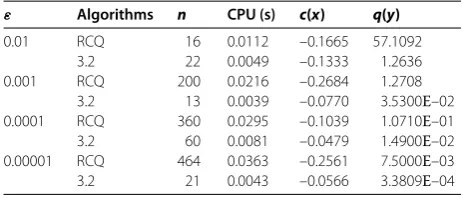
We setxn+–xn ≤εas the stop rule, and letN= ,M= ,g=I,D˜n=I, forn≥.
Using the methods in Section ., we compare Algorithm . with the relaxed CQ algo-rithm (RCQ) in [], with differentεand initial values. The results can be seen in Table . We see that the proposed methods in this paper behave better.
5 Concluding remarks
Table 1 The comparison between the results of preconditioning and relaxed CQ algorithms
ε Algorithms n CPU (s) c(x) q(y)
0.01 RCQ 16 0.0112 –0.1665 57.1092
3.2 22 0.0049 –0.1333 1.2636
0.001 RCQ 200 0.0216 –0.2684 1.2708
3.2 13 0.0039 –0.0770 3.5300E–02
0.0001 RCQ 360 0.0295 –0.1039 1.0710E–01
3.2 60 0.0081 –0.0479 1.4900E–02
0.00001 RCQ 464 0.0363 –0.2561 7.5000E–03
3.2 21 0.0043 –0.0566 3.3809E–04
method, variable modulus method and relaxed method, two modified projection algo-rithms for solving the GSFP and some approximate methods for algorithm executing have been presented. The numerical results show that by preconditioning method, the conver-gence speed of CQ algorithm can be improved, but the way to obtain variable stepsize in the paper is inexact. To continue to improve it or combine it with the methods in [] and [] is another interesting subject.
Competing interests
The authors declare that they have no competing interests.
Authors’ contributions
The authors take equal roles in deriving results and writing of this paper. All authors read and approved the final manuscript.
Author details
1The Second Training Base, Naval Aviation Institution, Huludao, 125001, China.2Department of Mathematics,
Shijiazhuang Mechanical Engineering College, Shijiazhuang, 050003, China. 3Department of Mathematics and Information, Hebei Normal University, Shijiazhuang, 050024, China.
Acknowledgements
The authors would like to thank the associate editor and the referees for their comments and suggestions. This research was supported by the National Natural Science Foundation of China (11071053).
Received: 14 February 2014 Accepted: 17 October 2014 Published:31 Oct 2014
References
1. Chen, K: Matrix Preconditioning Techniques and Applications. Cambridge University Press, New York (2005) 2. Piana, M, Bertero, M: Projected Landweber method and preconditioning. Inverse Probl.13, 441-463 (1997) 3. Strand, ON: Theory and methods related to the singular-function expansion and Landweber’s iteration for integral
equations of the first kind. SIAM J. Numer. Anal.11, 798-824 (1974) 4. Auslender, A: Optimisation: Méthodes Numérique. Masson, Paris (1976)
5. Dafermos, S: Traffic equilibrium and variational inequalities. Transp. Sci.14, 42-54 (1980)
6. Bertsekas, PD, Gafni, EM: Projection methods for variational inequities with application to the traffic assignment problem. Math. Program. Stud.17, 139-159 (1982)
7. Marcotte, P, Wu, JH: On the convergence of projection methods: application to the decomposition of affine variational inequalities. J. Optim. Theory Appl.85, 347-362 (1995)
8. Fukushima, M: A relaxed projection method for variational inequalities. Math. Program.35, 58-70 (1986) 9. Yang, Q: The revisit of a projection algorithm with variable steps for variational inequalities. J. Ind. Manag. Optim.1,
211-217 (2005)
10. He, BS: Inexact implicit methods for monotone general variational inequalities. Math. Program.86, 199-217 (1999) 11. Noor, MA, Wang, YJ, Xiu, N: Projection iterative schemes for general variational inequalities. J. Inequal. Pure Appl.
Math.3, Article 34 (2002)
12. Santos, PSM, Scheimberg, S: A projection algorithm for general variational inequalities with perturbed constraint sets. Appl. Math. Comput.181, 649-661 (2006)
13. Muhammad, AN, Abdellah, B, Saleem, U: Self-adaptive methods for general variational inequalities. Nonlinear Anal.
71, 3728-3738 (2009)
14. Qu, B, Xiu, N: A note on the CQ algorithm for the split feasibility problem. Inverse Probl.21, 1655-1665 (2005) 15. Byrne, C: A unified treatment of some iterative algorithms in signal processing and image reconstruction. Inverse
Probl.20, 103-120 (2004)
16. Dolidze, Z: Solution of variational inequalities associated with a class of monotone maps. Èkon. Mat. Metody18, 925-927 (1982)
17. He, B, He, X, Liu, H, Wu, T: Self-adaptive projection method for co-coercive variational inequalities. Eur. J. Oper. Res.
18. Facchinei, F, Pang, JS: Finite-Dimensional Variational Inequality and Complementarity Problems, vol. I. Springer, New York (2003)
19. Facchinei, F, Pang, JS: Finite-Dimensional Variational Inequality and Complementarity Problems, vol. II. Springer, New York (2003)
20. Yao, YH, Postolache, M, Liou, YC: Strong convergence of a self-adaptive method for the split feasibility problem. Fixed Point Theory Appl.2013, 201 (2013)
21. Yao, YH, Yang, PX, Kang, SM: Composite projection algorithms for the split feasibility problem. Math. Comput. Model.
57, 693-700 (2013)
22. Yao, YH, Liou, YC, Shahzad, N: A strongly convergent method for the split feasibility problem. Abstr. Appl. Anal.2012, Article ID 125046 (2012)
23. Mohammad, E, Abdul, L: General split feasibility problems in Hilbert spaces. Abstr. Appl. Anal.2013, Article ID 805104 (2013)
24. Censor, Y, Elfving, T: A multiprojection algorithm using Bregman projections in a product space. Numer. Algorithms8, 221-239 (1994)
25. Byrne, C: Iterative oblique projection onto convex sets and the split feasibility problem. Inverse Probl.18, 441-453 (2002)
26. Wang, PY, Zhou, HY: A preconditioning method of the CQ algorithm for solving the extended split feasibility problem. J. Inequal. Appl.2014, 163 (2014). doi:10.1186/1029-242X-2014-163
27. Yang, Q: On variable-step relaxed projection algorithm for variational inequalities. J. Math. Anal. Appl.302, 166-179 (2005)
28. López, G, Martín-Márquez, M, Wang, F, Xu, H-K: Solving the split feasibility problem without prior knowledge of matrix norms. Inverse Probl.28, 085004 (2012)
29. Wang, Z, Yang, Q, Yang, Y: The relaxed inexact projection methods for the split feasibility problem. Appl. Math. Comput.217, 5347-5359 (2011)
30. Yang, Q: The relaxed CQ algorithm solving the split feasibility problem. Inverse Probl.20, 1261-1266 (2004) 10.1186/1029-242X-2014-435