Iterative PSO Algorithms for GRAP Problems

2019 International Conference on Artificial Intelligence, Control and Automation Engineering (AICAE 2019) ISBN: 978-1-60595-643-5

Iterative PSO Algorithms for GRAP Problems

Fang LU

and Dong-kui LI

1

Faculty of Mathematics Science School, Baotou Teachers College, Baotou, Inner Mongolia, China 014030

2_{Editorial Department of Journal, Baotou Teachers College, Baotou, Inner Mongolia, China 014030}

*Corresponding author

Keywords: Mixed components, The reliability redundancy allocation problem, Particle swarm optimization algorithm, Encoding, Optimal solution.

Abstract. This paper studies the grap problems of two-state, in which the subsystem allows components to be mixed (i.e. the subsystem selects components from several types of heterogeneous components, and the number of selected components types >=1). Each component has a fixed reliability, weight and price, and determines the number of selected components, so that the system has the greatest reliability under the given cost and weight constraints. The coding method of the solution is that the number of elements of each type of subsystem is a variable, and the whole system is arranged in the order of subsystems to form row vectors. An iterative particle swarm optimization algorithm with fixed compression coefficient and dynamic inertia weight is constructed to solve the problem. Typical improved fyffe problems are tested, and the optimal solutions are obtained, which are consistent with the results given by the substitution constraint method. The pso algorithm presented in this paper can effectively solve the grap problem which is allowed to mix components in subsystems.

Introduction

There are many literature on reliability redundancy allocation problem (rap)[1]. According to the existing research results, the main methods to study rap are dynamic programming method [2], substitution constraints method [3], integer programming method [4], variable neighborhood descent method [5], improved substitution constraints method [6], IS method [7]; and genetic algorithm, ant colony algorithm, particle swarm optimization and other post-heuristic algorithms [8-26]. From the point of view of whether different kinds of components are allowed to mix in the subsystems studied, the literature on rap can be divided into two categories: the subsystems studied do not allow components to mix and the subsystems studied allow different types of components to mix (grap problem). Among them, the improved substitution constraint method [6] gives all the optimal solutions of 33 test cases, while other methods do not give all the optimal solutions of test cases, especially the post-heuristic algorithm.

In this paper, the constructed particle swarm optimization (pso) algorithm is used to solve 33 typical test cases, and all the optimal solutions of the test problem are given. The results are consistent with those given by the improved substitution constraint method [6].

Hypothesis and Model

Hypothesis

Hypothesis 1 components and systems have and only have two states, i.e. normal working state and failure state;

Hypothesis 2 the properties of components, i.e. reliability, price and weight, are known and determined;

Hypothesis 3 different types of components are allowed to be mixed in a subsystem;

The system S studied in this paper is composed of Si subsystems in series, i=1,2,... n; each subsystem is composed of several parallel components of different types of mi (at least one component of each subsystem works normally), each component i has reliability rij, price cij, weight wij; requirements: under the condition that the total weight and total cost of the system do not exceed W0 and C0 respectively, the reliability of the system is maximized by determining the redundancy of components, the mathematical formulas are as follows:

max 𝑅_𝑠 = ∑𝑛 𝑅_𝑖

𝑖=1 . (1)

s.t. ∑𝑛_𝑖=1𝐶_𝑖 ≤ 𝐶₀ .

∑𝑛 𝑊_𝑖 ≤ 𝑊₀

𝑖=1 . (2)

Where Ri, Ci and Wi are subsystem i’s reliability, cost and weight respectively.

Algorithm

Data Storage and Coding Method

Reliability, price and weight data of each component need to be stored. Specific methods are as follows: the reliability, price and weight of components in each subsystem are arranged in order of component indexes (e.g. subscripts), and processed into the same length (subsystems with fewer components, all kinds of data of missing component bits are made up of 0), then row vectors are formed for storage. For example, in a typical example (see Section 3, Table 1 for specific data), component reliability, component price and component weight vector are:

P=[0.9,0.93,0.91,0.95,0.95,0.94,0.93,0,0.85,0.9,0.87,0.92,0.83,0.87,0.85,0,0.94,0.93,0.95,0,0.99, 0.98,0.97,0.96,0.91,0.92,0.94,0,0.81,0.90,0.91,0,0.97,0.99,0.96,0.91,0.83,0.85,0.90,0,0.94,0.95,0.96 ,0,0.79,0.82,0.85,0.9,0.98,0.99,0.97,0,0.9,0.92,0.95,0.99];

C=[1,1,2,2,2,1,1,0,2,3,1,4,3,4,5,0,2,2,3,0,3,3,2,2,4,4,5,0,3,5,6,0,2,3,4,3,4,4,5,0,3,4,5,0,2,3,4,5,2,3,2, 0,4,4,5,6];

W=[3,4,2,5,8,10,9,0,7,5,6,4,5,6,4,0,4,3,5,0,5,4,5,4,7,8,9,0,4,7,6,0,8,9,7,8,6,5,6,0,5,6,6,0,4,5,6,7,5,5, 6,0,6,7,6,9];

Similarly, the redundancy variables of each component of the system constitute a sub-vector of the same length according to the subsystem (no optional data bit is added to 0), and then a row vector is formed as the solution vector, that is, a particle in the pso algorithm (the encoding of the solution).

New Solution Generation Algorithms

The symmetric bit transformation technique is used to generate the new solution. The specific algorithm is as follows:

New solution X generation algorithm:

Setp0 gives the initial solution X0 that meets the above coding requirements.

Step1 for each component i of the initial solution X0, for the random number Rand generated by uniform distribution of (0,1) intervals, if Rand >= 0.5, the position i bit of X0 is added with a random number and integrates. Otherwise, the symmetric bit of X0 is subtracted from a random number and integrates; and note that the data bit complemented with 0 is unchanged when encoding.

Step2 algorithm terminates.

Construction of Fitness Function

as follows:

max 𝑓(𝑋, 𝐶, 𝑊) = {

𝑅_𝑠 𝑖𝑓𝐶 ≤ 𝐶₀, 𝑊 ≤ 𝑊₀

𝑅𝑠∗ min ((_𝐶𝐶

0)

𝛼 , (_𝑊𝑊

0)

𝛽

) 𝑜𝑡ℎ𝑒𝑟𝑤𝑖𝑠𝑒 (3)

Iterative PSO Algorithms

The improved pso algorithm is called iterative pso algorithm. After iterating the speed and position of particle swarm optimization algorithm, the velocity and position iteration formulas are used to deal with the non-conforming particles again, which improves the convergence of the original basic particle swarm optimization algorithm. The algorithm is described as follows:

Iterative pso algorithm (pseudo-matlab code)

Step0 (initialization) determines the initial solution X0, and stores the known data in a vector manner according to the coding format requirements: component reliability vector P, component price vector C, component weight vector W, and compression coefficient C1 = C2 = 1.4962. Let V=zeros (n1, n2), where n1 is the solution vector dimension and n2 is the number of population particles. A = B = zeros (n1, n2), CA = CB = zeros (1, n2), Z = zeros (1, nt), nt is the total number of cycles; E = X0, E stores the optimal solution.

Step1 generates n2 new solutions according to the new solution generation algorithm and stores them in matrix A; calculates the fitness value of each solution in matrix CA; generates n2 new solutions according to the new solution generation algorithm and stores them in matrix B; and calculates the fitness value of each solution in matrix CB (where B stores the initial local optimal solution of particles).

Step2 for t = 1: nt

The dynamic inertia weight wt=0.9-0.5*(t-1)/nt is determined.

The system cost TC and system weight TW corresponding to the optimal solution E are determined and the fitness value e corresponding to the optimal solution E is calculated.

Step2.1 For each particle in population A, if the fitness value of population A is greater than that of corresponding particle in population B, then the value of population A is assigned to corresponding particle in population B.

If the fitness of population B particle is greater than the fitness of optimal solution e, then population B particle is assigned to the current optimal solution E.

Step2.2 For each particle of the population j = 1:n2 for each component of a particle i = 1:n1

Calculation:

𝑉(i, j) = 𝑤_𝑡𝑉(𝑖, 𝑗) + 𝑐1 ∗ 𝑟𝑎𝑛𝑑 ∗ (𝐵(𝑖, 𝑗) − 𝐴(𝑖, 𝑗)) + 𝑐2 ∗ 𝑟𝑎𝑛𝑑(𝐸(1, 𝑗) − 𝐴(𝑖, 𝑗)) (4)

𝐴(i, j) = round (𝐴(i, j) + 𝑉(i, j)) . (5)

If A(i,j)<1, then let A(i,j)=0 . (6) Step 2.3 judges whether the updated population A satisfies the constraints. If it satisfies the constraints, go to step 2.4; otherwise, update population A according to formula (4) - (6) until the condition is satisfied. Note that: to keep the position of 0 in the solution is still zero.

Step 2.4 recalculates the fitness CA and CB of population A and B. Step2.5 Z (:, t) = Reliability of the optimal solution.

Step3 gives the optimal solution E, the reliability of the optimal solution E, the optimal solution corresponds to the system cost, the optimal solution corresponds to the system weight, and draws the convergence curve.

For the improved fyffe [3,11] problem, the component types, reliability, price and weight data of 14 subsystems are listed in Table 1. The cost constraints of the system are 130 units, and the weight constraints of the system change from 159 units to 191 units. The optimal solutions and corresponding reliability of 33 grap problems are calculated.

Table 1. Known data for the improved fyffegrap problem.

Sub system

Optional component type

1 2 3 4

R C W R C W R C W R C W

1 0.90 1 3 0.93 1 4 0.91 2 2 0.95 2 5 2 0.95 2 8 0.94 1 10 0.93 1 9 * * * 3 0.85 2 7 0.90 3 5 0.87 1 6 0.92 4 4 4 0.83 3 5 0.87 4 6 0.85 5 4 * * * 5 0.94 2 4 0.93 2 3 0.95 3 5 * * * 6 0.99 3 5 0.98 3 4 0.97 2 5 0.96 2 4 7 0.91 4 7 0.92 4 8 0.94 5 9 * * * 8 0.81 3 4 0.90 5 7 0.91 6 6 * * * 9 0.97 2 8 0.99 3 9 0.96 4 7 0.91 3 8 10 0.83 4 6 0.85 4 5 0.90 5 6 * * * 11 0.94 3 5 0.95 4 6 0.96 5 6 * * * 12 0.79 2 4 0.82 3 5 0.85 4 6 0.90 5 7 13 0.98 2 5 0.99 3 5 0.97 2 6 * * * 14 0.90 4 6 0.92 4 7 0.95 5 6 0.99 6 9

The configuration of micro-computer is Intel (R) Core (TM) [email protected] 3.20 Ghz, 8GB of memory, 600Gb of hard disk, Windows 10 professional edition, and the programming software is MATLAB R2015b.

The parameters of the algorithm are set as follows: n1 =14, C1 = C2 = 1. 4962, C0 = 130, W0 = 159,... 191, n2 = 200, nt =500, α=β=2. Running the algorithm 50 times in each case, recording the maximum reliability and the optimal solution, the minimum reliability and the average reliability, etc. See Table 2-3 for details.

Table 2. Maximum, Minimum and Average Reliability for each grap Problem Running 50 Times.

C0 W0 Max Reliab. Min.Reliab. Aver.Reliab TC,TW of optimal solution

130 191 0.98681 0.98305 0.98552 TC=130 TW=191

130 190 0.98642 0.98395 0.98539 TC=130 TW=190 130 189 0.98592 0.97871 0.98456 TC=130 TW=189

130 188 0.98358 0.97832 0.98263 TC=130 TW=188

130 187 0.98469 0.97774 0.98247 TC=130 TW=187

130 186 0.98418 0.97742 0.98315 TC=129 TW=186

130 185 0.98351 0.97666 0.98157 TC=130 TW=185

130 184 0.98299 0.97518 0.98134 TC=130 TW=184

130 183 0.98226 0.97591 0.98060 TC=129 TW=183

130 182 0.98152 0.97960 0.98011 TC=130 TW=182 130 181 0.98103 0.97484 0.98026 TC=129 TW=181 130 180 0.98029 0.97411 0.97872 TC=128 TW=180 130 179 0.97951 0.97484 0.97846 TC=126 TW=179 130 178 0.97840 0.97259 0.97693 TC=125 TW=178 130 177 0.97760 0.97391 0.97612 TC=126 TW=177 130 176 0.97669 0.97336 0.97559 TC=124 TW=176

130 175 0.97571 0.97143 0.97480 TC=125 TW=175

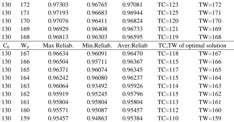
130 172 0.97303 0.96765 0.97081 TC=123 TW=172 130 171 0.97193 0.96683 0.96944 TC=125 TW=171

130 170 0.97076 0.96411 0.96824 TC=120 TW=170

130 169 0.96929 0.96408 0.96733 TC=121 TW=169 130 168 0.96813 0.96303 0.96595 TC=119 TW=168 C0 W0 Max Reliab. Min.Reliab. Aver.Reliab TC,TW of optimal solution 130 167 0.96634 0.96091 0.96470 TC=118 TW=167 130 166 0.96504 0.95711 0.96367 TC=115 TW=166 130 165 0.96371 0.96074 0.96345 TC=117 TW=165 130 164 0.96242 0.96080 0.96237 TC=115 TW=164 130 163 0.96064 0.93492 0.95926 TC=114 TW=163

130 162 0.95919 0.95245 0.95796 TC=115 TW=162

130 161 0.95804 0.95804 0.95804 TC=113 TW=161

130 160 0.95571 0.95087 0.95457 TC=112 TW=160

130 159 0.95457 0.94863 0.95384 TC=110 TW=159

Table 3. Optimal solutions for each grap problem with maximum reliability of 50 runs.

C0 W0 Optimal Solution Corresponding to Maximum Reliability

Total time [seconds] 130 191 0030 2000 0003 0040 0300 0200 3000 4000 1100 0120 0020 4000 2000 0011 1364.70 130 190 0030 2000 0003 0040 0300 0200 3000 4000 2000 0120 0020 4000 1100 0011 1328.01 130 189 0030 2000 0003 0040 0300 0200 3000 4000 0110 0120 1010 4000 2000 0011 1344.18 130 188 0030 2000 0003 0040 0300 0200 3000 4000 0110 0210 1010 4000 1100 0011 1210.99 130 187 0030 2000 0003 0040 0300 0200 3000 4000 1010 0210 1010 4000 0200 0011 1246.01 130 186 0030 2000 0003 0030 0300 0200 3000 4000 0110 0120 0020 4000 0200 0011 1153.11 130 185 0030 2000 0003 0040 0300 0200 3000 4000 0110 0210 1010 4000 0200 0020 1219.28 130 184 0030 2000 0003 0030 0300 0200 3000 4000 0020 0120 0020 4000 0200 0011 1146.26 130 183 0030 2000 0003 0030 0300 0200 3000 4000 0020 0210 0020 4000 0200 0011 1182.01 130 182 0030 2000 0003 0030 0300 0200 3000 4000 0020 0030 0020 4000 0200 0020 1107.43 130 181 0030 2000 0003 0030 0300 0200 3000 4000 0020 0120 0020 4000 0200 0020 1140.84 130 180 0030 2000 0003 0030 0300 0200 3000 4000 0020 0120 0020 4000 0200 0020 1174.02 130 179 0030 2000 0003 0030 0300 0200 3000 4000 0020 0210 1010 4000 0200 0020 1267.64 130 178 0030 2000 0003 0030 0300 0200 3000 4000 0020 0300 1010 4000 0200 0020 1282.18 130 177 0030 2000 0003 0030 0300 0200 3000 2010 0020 0210 1010 4000 0200 0020 2119.07 130 176 0030 2000 0003 0030 0300 0200 0020 4000 0020 0210 1010 4000 0200 0020 2102.65 130 175 0030 2000 0003 0030 0300 0200 1010 4000 0020 0210 0020 4000 0200 0020 1965.67 130 174 0030 2000 0003 0030 0300 0200 1010 4000 0020 0210 1010 4000 0200 0020 2004.91 130 173 0030 2000 0003 0030 0300 0200 1010 4000 0020 0300 1010 4000 0200 0020 1972.76 130 172 0030 2000 0003 0030 0300 0200 1010 2010 0020 0210 1010 4000 0200 0020 2384.23 130 171 0030 2000 0003 0030 0300 0200 1010 2010 0020 0300 1010 4000 0200 0020 2465.62 130 170 0030 2000 0003 0030 0300 0200 1010 2010 0020 0300 2000 4000 0200 0020 2876.94 130 169 0030 2000 0003 0030 0300 0200 2000 2010 0020 0300 1010 4000 0200 0020 3079.50 130 168 0030 2000 0003 0030 0300 0200 2000 2010 0020 0300 2000 4000 0200 0020 3262.42 130 167 0030 2000 0003 0030 0200 0200 1010 2010 0020 0300 2000 4000 0200 0020 3280.07 130 166 0030 2000 0002 0030 0300 0200 1010 2010 0020 0300 2000 4000 0200 0002 1367.99 130 165 0030 2000 0003 0030 0200 0200 2000 2010 0020 0300 2000 4000 0200 0002 1301.75 130 164 0030 2000 0002 0030 0300 0200 2000 2010 0020 0300 2000 4000 0200 0020 1302.63 130 163 0030 2000 0002 0030 0200 0200 1010 2010 0020 0300 2000 4000 0200 0020 1528.79 130 162 0030 2000 0002 0030 0200 0200 2000 2010 0020 0300 1010 4000 0200 0020 1386.44 130 161 0030 2000 0002 0030 0200 0200 2000 2010 0020 0300 2000 4000 0200 0020 1323.27 130 160 0030 2000 0002 0030 0200 0200 2000 3000 0020 0300 1010 4000 0200 0020 1475.97 130 159 0030 2000 0002 0030 0200 0200 2000 3000 0020 0300 2000 4000 0200 0020 1319.12

first type and one component of the second type, and the tenth subsystem one type 2 component and two type 3 components are selected, and one type 3 component and one type 4 component are selected for the 14 subsystems. The results are consistent with those obtained by the improved substitution constraint method [6]. It is the best optimization result for these grap problems at present.

Conclusion

An improved pso algorithm with iteration is used to solve the extended fyffe reliability redundancy allocation problem. This kind of optimization problem allows the subsystem to have component mixing, which has a larger search space than the similar reliability redundancy allocation problem that does not allow component mixing. The simulation results show that the algorithm is effective and fast, and has certain practical application value. At present, the main problem of the algorithm is that the initial solution in the test case is not easy to obtain, which is worth further exploration.

Acknowledgement

This research was financially supported by the Inner Mongolia Natural Science Foundation (2018MS06031), and Inner Mongolia University Science Research Project (NJZY17290).

References

[1] D. W. Coit, E. Zio, The evolution of system reliability optimization, Reliab. Eng. Syst. Saf. (2018) doi: https://doi.org/10.1016/j.ress.2018.09.008.

[2] D. E. Fyffe, W. W. Hines, N. K. Lee, System reliability allocation and a computational algorithm, IEEE Trans. Reliab. 17(1968)64-69.

[3] Y. Nakagawa, S. Miyazaki, Surrogate constraints algorithm for reliability optimization problems with two constrains, IEEE Trans. Reliab. 30(1981)175-180.

[4] D. W. Coit, J. C. Liu, System reliability optimization with k-out-of-n subsystems, Int. J. Reliab., Qua. Saf. Eng. 7(2000):129-142.

[5] Y. C. Liang, C. C. Wu, A variable neighborhood descent algorithm for the redundancy allocation problem, IEMS 4(2005)94-101.

[6] J. Onishi, S. Kimura, R.J.W. James, et al, Solving the redundancy allocation problem with a mix of components using the improved surrogate constraint method, IEEE Trans. Reliab. 56(2007)94-101.

[7] K. H. Chang, P. Y. Kuo, An efficient simulation optimization method for the generalized redundancy allocation problem, Euro. J. Oper. Res. 265(2018) 1094 -1101.

[8] D.W. Coit, A. E. Smith, Reliability optimization of series-parallel systems using a genetic algorithm, IEEE Trans.Reliab.45(1996)254-260.

[9] Z. J. Xu, C. W. Ma, Q. Z. Mei, et al, Solving a system reliability optimization problem with genetic algorithms, J. Tsinghua Unive. (Natu. Sci. Edit.), 84(1998)54-57.

[10] T.Z. Zhang, C. X. Teng, Z.G. Han, Application of genetic algorithms in system reliability optimization, Contr. Deci.17(2002):378-384.

[12] H. Gholinezhad, A. Z. Hamadani, A new model for the redundancy allocation problem with component mixing and redundancy strategy, Reliab. Eng. Syst. Saf. 102(2017)164:66-73.

[13] W.C. Yeh. A two-stage discrete particle swarm optimization for the problem of multiple multi-level redundancy allocation in series systems, Expert Syst .Appl.36(2009)9192-9200.

[14] M.S. Chern, On the computational complexity of reliability redundancy allocation in a series system, Oper. Res. Lett.11(1992)309-315.

[15] G. Mitsuo, S.Y. Young, Soft computing approach for reliability optimization: state- of-the art survey, Reliab. Eng. Syst. Saf. 91(2006) 1008-1026.

[16] G. Walter, C. Pflug, R. Anarzej, Configurations of series-parallel networks with maximum reliability, Working Paper, WP-93-60.

[17] R.E. Bellman, Dynamic Programming, first ed., Princeton University Press, Princeton, 1957.

[18] R.E. Bellman, E. Dreyus, Dynamic programming and reliability of multi-component devices, Oper. Res. 6(1958)200-206.

[19] R.E. Bellman,E. Dreyus, Applied Dynamic Programming, Princeton University Press, Princeton, 1962.

[20] N. Beji, B. Jarboui, M. Eddaly, et al, A hybrid particle swarm optimization algorithm for the redundancy allocation problem, J. Comput. Sci. (2010)159-167.

[21] A.E. Jahromi, M. Feizabadi, Optimization of multi-objective redundancy allocation problem with non-homogeneous components, Comput. Ind. Eng. 108(2017)111-123.

[22] D. K. Li, Particle swarm optimization for reliability optimization of s-p networks with single-objective and multi-condition constraints, Modern Electron. Technol. 41(2018)89-92.

[23] D. K. Li, H. Dong, Reliability optimization of s-p network with parallel non-identical components, Yinshan Acad. J. (Natu. Sci. Edit.)30(2016)35-41.

[24] D. K. Li, Wulantuya, Y. L. Zhu, Comparative study on intelligent algorithm for reliability optimization of series parallel networks based on MATLAB, Electron. Commer. (2015)58-60.

[25] W. C. Yeh, A new exact solution algorithm for a novel generalized redundancy allocation problem[J]. Inform. Sci. 408(2017):182-197.