Synthesis of Parallel Robots Optimal Motion Trajectory Planning Algorithms

2018 IX International Conference on Optimization and Applications (OPTIMA 2018) ISBN: 978-1-60595-587-2

Synthesis of Parallel Robots Optimal Motion Trajectory Planning

Algorithms

Sergey KHALAPYAN

_{, Larisa RYBAK}

,

Dmitry MALYSHEV

_{, and Viktoria KUZMINA}

Stary Oskol Technological Institute (Branch) N.a. A.A. Ugarov NUST MISiS, Makarenko Microdistrict 42, 309516 Stary Oskol, Russia

BSTU named after V. G. Shoukhov, Kostyukov str. 46, 308012 Belgorod, Russia Corresponding author

parallel robot, optimal trajectory, working area.

Abstract. _{The article considers the problem of planning the optimal trajectory of the tripod robot}

movement. The movement of the output link includes working displacements that are performed for the purpose of machining the workpiece and are completely determined by the surface of the workpiece, as well as the movement of the tool to the beginning of the next stage of processing, which can be relatively free, however, taking into account working area and workpiece surface limitations. The working area is limited by the range of permissible lengths of the drive links and the sign of the Jacobian. Additional restrictions are introduced, related to the dimensions of the workpiece. Chebyshev’s metric makes a significant ambiguity in the choice of the trajectory. Therefore, it is proposed to supplement the original objective function with the Euclidean metric taken with a small weighting factor. Optimization was carried out with restrictions on the size of the working area and workpiece.

Introduction

The task of controlling a robot machine of a parallel structure includes two related subtasks: planning an optimal trajectory of motion and its implementing. The realization of the chosen tra jectory of motion is carried out by standard methods of control theory and considered, in particular, in [8]. The tra jectory of the mechanism is largely determined by the tasks posed. Motion planning is an important task for obstacles bending by parallel robots. The boundaries of the working area and the singularity can be considered as obstacles in our case. Two main methods of planning the movement are known in the present time: the potential fields and the space configuration method. In the first case, the positive potential is associated with the goal and the negative with the obstacle. The movement of the output link depends on the interaction of these fields. This method has never been used to plan the movement of parallel robots. Research shows that local minimum problems, which are the main problems when working with a potential field, are more than real for planning the movement of a parallel robot.

The preparatory step of space configuration method is a determination of the free space in the form of cells set (cell decomposition method) or possible positions (the roadmap method). When

1

2

Keywords:

a definition is specified, the motion planning is a connection of the endpoints and the start points using cells or possible positions.

This method was extended for use with a closed trajectory [17, 18, 16], but the main problem of the method is a random selection of variables in the node region has a zero probability of satisfying expressions. Moreover, the singularity and self-intersections are not taken into account usually in this method. The one working method for parallel robots is the probabilistic roadmap method proposed by [1]. It improved the algorithm for determining possible positions by using the robot structure, and a very effective algorithm was obtained. But the local planner does not take into account the singularity and multivariance of the local kinematics solution, which can prevent further use of the trajectory.

The movement can be carried out relatively freely along some arbitrary trajectory, taking into account the constraints determined by the working area of the mechanism and the surface of the workpiece for considering the task of positioning - moving the tool to the beginning of the next stage of processing. The duration of positioning affects the total processing time of the product, so it should be minimized as much as possible. Since the positioning duration is determined by the duration of operation of the actuators of the mechanism necessary for the corresponding movement of the tool, it is advisable to carry out its optimization in the space of input coordinates.

The considered mechanism (Fig. 1.) consists of three rods of variable length hinged fixed by one of its ends at the vertices of an equilateral triangle A1A2A3 motionlessly located in the horizontal

plane. The second end of each rod is also hinged fixed to the vertices of another equilateral triangle

B1B2B3. The hinges allow free movement of the second triangle (movable platform) relative to the

first (base) in the horizontal plane at changing the rod lengths. The lengths of the rods l1, l2, l3

describe the state of the input link of the mechanism and can be changed independently by drive electric motors. The state of the output link of the mechanism is described by the position of the moving platform geometric center (linear coordinates x, y) and the angle of its rotation φ around the vertical axis.

Schemes, coupling equations, and solutions of the inverse problem of positions are presented in [12, 15]. In the article [3], the dependence of the location of singularity zones on the values of the determinant of the Jacobi matrix and the geometric parameters of the output link was obtained. In paper [7], the dynamic stiffening has been investigated with considering the effect of axial forces on the lateral vibration of a 3-RPR parallel manipulator with three flexible intermediate links. If the joint clearances of the joints of a manipulator are considered, an unconstrained motion of the end-effector can be computed. Paper [6] presents how this unconstrained motion can be determined for a planar 3-RPR manipulator. It is shown that when clearances are considered, the singularity curves normally found in the workspace of such a manipulator become singular zones. Optimization of the positioning trajectory is a complex scientific task of the mechanism output link safe motion trajectoryC0C1CK determination on a uniform discrete grid ensuring a minimum

of the total positioning time t. Safe motion is the movement at a distance not less than the specified from the boundaries of the working area and mechanism singularity zones[2], determined by its geometric characteristics [9, 14] and also from the surface of the workpiece. The described limitations can be specified both in the form of corresponding inequalities and in the form of an array of discrete points forbidden or allowed to be included in the trajectory.

Figure 1. Planar 3-RPR mechanism

As shown in [14] and [9], the output coordinates x, y, φ (Fig. 2) of this mechanism (working space) are limited by the range of permissible lengths of the drive links and area where the Jacobian sign is constant.

Figure 2. The workspace of the planar 3-RPR mechanism in coordinates (x, y, φ)

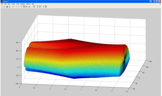
The transformation (x, y, φ)→(l1, l2, l3), which is, in fact, the solution of the inverse kinematic

Figure 3. The workspace of the planar 3-RPR mechanism in coordinates (l1, l2, l3)

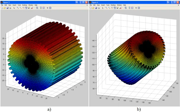
Figure 4. Additional restrictions associated with the overall dimensions of the workpiece: a) in the coordinates (x, y, φ); b) in the coordinates (l1, l2, l3)

Positioning Trajectories Duration

An arbitrary positioning trajectory can be represented as a set of small movements (steps) during which the drives of translational pairs operate at a constant speed and the movement in the space of the input coordinates is rectilinear. In order to reduce the duration of such small movements, the maximum rate of change in the lengths of the drive links at each step must correspond to the maximum possible. In this case, the duration of each step is uniquely determined

by the largest in absolute value projection of the vector of the corresponding small movement onto the coordinate axes. In other words, the duration of the positioning is proportional to the sum of the lengths of the individual steps defined according to Chebyshev’s metric:

t= 1

vmax n

X

i=1

ρi (1)

where ρi = maxj∈{1,2,..,m}|lj,i −ll,i−1| — according to Chebyshev distance between the points of

beginningAi−1(l1,i−1, l2,i−1, .., lm,i−1) and endAi(l1,i, l2,i, .., lm,i) of the istep; m – number of input

coordinates (for the considered mechanism m = 3);vmax – the maximum rate of change in the

length of the link.

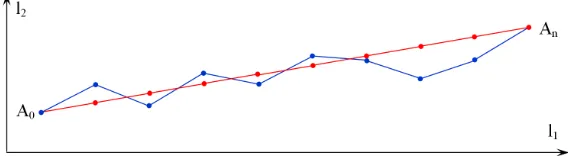
However, the direct use of this parameter as an objective function for the optimization of the positioning trajectory is impractical, since Chebyshev’s metric introduces a significant ambiguity into the trajectory selection. From Fig. 5 it can be seen that for the optimal trajectory, in this case, it is not excluded groundless speed change and even reverse of the drives.

Figure 5. An example of the optimal duration positioning trajectories

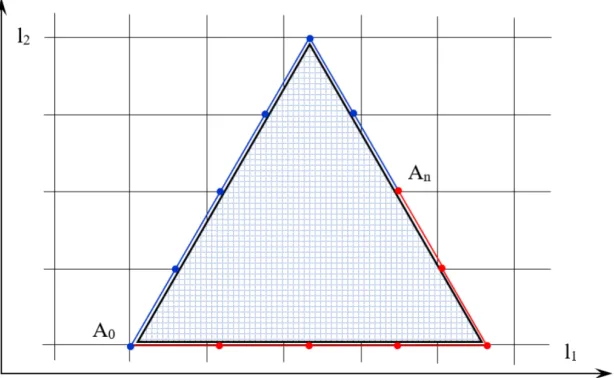
On the other hand, the use of the “usual” trajectory length (the sum of the Euclidean lengths of all steps) as objective functions is also unacceptable. The duration of positioning, in this case, may be far from optimal. Thus, the loss of time when selecting the red trajectory of motion on Fig. 6 is

1−sin 60◦

Figure 6. An example of the optimal length of the trajectories with different durations of posi-tioning

Therefore, it is proposed to supplement the primary objective function with the Euclidean metric taken with some small weighting coefficient:

k

X

i=1



 max

j∈{1,2,..,m}|lj,i−ll,i−1|+α

v u u t m X i=1

(lj,i−ll,i−1)2



→min (3)

Optimization should be carried out with restrictions on the size of the workspace and (if neces-sary) the workpiece. Each point of the trajectoryCiwith the coordinates (xi, yi, φi) ( or (li,1, li,2, li,3))

must satisfy the inequalities:

lmin ≤li,1 =



 xi+

r

2(sinφi− √

3 cosφi) + √ 3 2 θ !2 +

yi− r

2( √

3 sinφi+ cosφi) + θ

2

2!0,5

≤lmax,

(4)

lmin ≤li,2 =



 xi+

r

2(sinφi+ √

3 cosφi)− √ 3 2 θ !2 +

yi+ r

2( √

3 sinφi−cosφi) + θ

2

2!0,5

≤lmax,

(5)

lmin ≤li,3 =

p

(xi −rsinφi)2+ (yi+rcosφi−θ)2 ≤lmax, (6)

J(x, y, φ) = 12√3θrsinφ(θ2−2θrcosφ+r2 −x2_i −y_i2)≤Jmin, (7)

where Θ, r are the known geometric parameters of the mechanism, lmin and lmax are the limiting

values of the rod lengths, taking into account the necessary remoteness from the boundaries of the working space[4, 5, 13], J(xi, yi, φi) and Jmin is the Jacobian and its minimum allowable value,

taking into account the necessary remoteness from points of singularity [14].

Since the workpiece has a complex surface in general, there are additional limitations associated with the need to bend the workpiece during positioning. It is advisable to specify them in the form of a binary matrix that determines on a uniform discrete grid the points that are allowed and forbidden for “visiting”.

In [10] methods of searching for the optimal trajectory of cargo movement by a crane are proposed on the basis of: genetic approach; algorithm of swarm intelligence; algorithm for decom-position of linear and angular coordinates; algorithm of a probabilistic roadmap; directed wave algorithm.

This methods, after some modification of the algorithms, which connected first of all with the absence of the gravitational vertical coordinate for the mechanisms parallel structure relative to which an array of the hypersurface of constraints was constructed in [10], as well as with another kind of objective function, can be used to solve the problem under consideration.

So, in the beginning, the hypersurface of constraints (in the particular case, equidistant) is constructed in the output coordinates, which provides the distance of the trajectory necessary for safe positioning from the surface of the workpiece and the boundaries of the working space of the mechanism.

Algorithms for Constructing the Hypersurface of Constraints

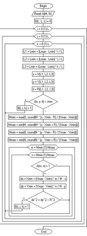
The algorithm for constructing the hypersurface of constraints (Fig. 7) provides:

1. Input of the initial information - a binary matrix A, describing the shape of the workpiece on a uniform discrete grid in the space of output coordinates of the mechanism.

2. Zeroing of the workspace B binary array, which defines the hypersurface of constraints on a uniform discrete grid in the space of input coordinates.

3. A cyclic change in the indices of the input coordinates i, j, k in the range 0...L is specified. 4. The corresponding input coordinates of the mechanismL1, L2, L3 are calculated by the formulas:

L1 =Lmin+ _Li(Lmax−Lmin), L2 =Lmin+ _Lj(Lmax−Lmin), L3 =Lmin+ k_L(Lmax−Lmin).

(8)

where Lmin and Lmax minimum and maximum length of the drive links, respectively.

5. The values of the output coordinates (x, y, φ) are determined on the basis of neural network functions [9], providing the solution of the direct kinematic analysis problem.

Figure 7. An algorithm for constructing constraints hypersurface

m= max0, roundMx−xmin−R xmax−xmin

...minM, roundMx−xmin+R xmax−xmin

n= max0, roundNy−ymin−R ymax−ymin

...minN, roundMy−ymin+R ymax−ymin

, (9)

where round() – rounding function to nearest integer, R a given distance from the hypersurface of constraints to the points of the binary matrix A that determine the contours of the workpiece,

xmin, xmax, ymin, ymax – limiting values of output coordinates.

8. If the next point (m, n) is forbidden

A(m, n) = 1 (10)

and the distance from it to the current point (x, y) is less than the specified

r

xmin+ m

M(xmax−xmin)−x

2 +

ymin+ n

N(ymax−ymin)−y

2

< R (11)

the value 1 is stored in an array of workspace B (as a result, the existing constraints are transferred to the input coordinates) and the transition to item 10 is performed.

9. The transition to the next iteration of item 7. 10. The transition to the next iteration item 3.

If, as a result of machining, there are no significant changes in the linear dimensions of the part, the described algorithm can be performed only once. If such changes occur, an additional correction of array B may be recommended to reduce the positioning time in accordance with the change in matrix A.

Positioning (with the exception of the initial one) is performed at the end of the next stage of the product processing (working displacement) and starts from a certain resolved point C0 into

which the tool is directly removed from the workpiece surface. Similarly, the end of the positioning (with the exception of the final one) should be at some authorized point of theCK, from which it

is supposed to carry the tool to the surface of the workpiece.

The remaining points of the trajectory C1. . . CK−1 should be chosen as a result of its

optimiza-tion. The initial family of random trajectories, each of which is a collection of successive rectilinear displacements (steps) from the point Ci to the point Ci+1, and provides a safe (with allowance for

restrictions) translation of the mechanism from the point C0 to the pointCK, can be constructed

by any of the methods listed above .

An algorithm of discrete local optimization [11] can be applied to each of these trajectories, which reduces to a sequential decrease in the length of steps as a result of multiple transfers of individual points. This technique is designed to reduce the total length of the trajectory, but as it is easy to show, its use will not lead to an increase in the duration of positioning, so the above objective function as a result of such optimization can be reduced.

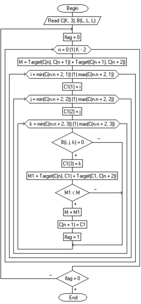
Its modification, suitable for use for the optimization of the positioning path, is shown in Fig. 8. The algorithm provides for a cyclic change in the position of the points Cn+1, each of which

ensures the minimization of the objective function in the section Cn...Cn+2 taking into account

the established limitations. The condition for the completion of the algorithm is the absence of changes in the route C0...CK as a result of the next iteration.

Step-by-step description of the algorithm:

1. The initial data are the binary array of the workspace B formed at the previous stage and the optimized trajectory consisting of the points C0...CK, each of which is given by three indices on

the uniform discrete grid of the input coordinates Cn,1, Cn,2, Cn,3.

Figure 8. Modified algorithm for discrete local optimization

M = max(|Ln,1−Ln+1,1|,|Ln,2−Ln+1,2|,|Ln,3−Ln+1,3|)

+ max(|Ln+2,1−Ln+1,1|,|Ln+2,2−Ln+1,2|,|Ln+2,3−Ln+1,3|)

+α

_q

(Ln,1−Ln+1,1)2+ (Ln,2−Ln+1,2)2+ (Ln,3−Ln+1,3)2

+ q

(Ln+2,1−Ln+1,1)2+ (Ln+2,2−Ln+1,2)2+ (Ln+2,3−Ln+1,3)2

,

(12)

where Ln,j — coordinates of an arbitrary point of the trajectory Cn, which are defined by the

relation:

Ln,j =Lmin+ Cn,j

L (Lmax−Lmin), (13)

5. The indices of the coordinates of point C1 vary in the ranges:

C11 =i= min(Cn,1, Cn+1,1, Cn+2,1)...max(Cn,1, Cn+1,1, Cn+2,1) C12 =j = min(Cn,2, Cn+1,2, Cn+2,2)...max(Cn,2, Cn+1,2, Cn+2,2), C13 =k = min(Cn,3, Cn+1,3, Cn+2,3)...max(Cn,3, Cn+1,3, Cn+2,3).

(14)

6. Point C1 is checked for belonging to the allowed part of the workspace: if

B(i, j, k)6= 0, (15)

the transition to item 9 is carried out.

7. Otherwise, the value M1 of the target function for the path section Cn→C1→Cn+2.

8. If M1 is less than the stored value of M, the following actions are performed: – the minimum of the objective function M = M1 is updated;

– the point Cn+1 is transferred to the point C1;

– the sign of the optimization is established f lag= 1. 9. The transition to the next iteration item 5.

10. The transition to the next iteration item 3.

11. If during the completed passage the trajectory was not optimized:

f lag = 0, (16)

the algorithm is completed. 12. Otherwise, go to item 2.

Results of Optimization

The optimized trajectory is formed in array C as a result of the algorithm execution. Let us illustrate the proposed method by the example of changing the lengths of two links (two-dimensional problem).

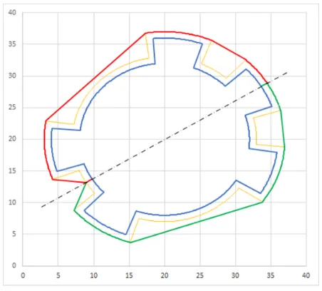
As a result of applying discrete local optimization, the original family of random trajectories is red, green and brown lines in Fig. 9 (the step size is greatly exaggerated) – will be reduced to two routes – the red and green lines in Fig. 10. It is obvious that their length is the same, however, as the calculation (Table 1) shows, positioning along the green trajectory takes 8.5% more time.

Conclusions

work-Figure 9. Positioning trajectories set and its optimization (the step size is greatly exaggerated)

Figure 10. Comparison of the trajectories after optimization

operation of the drives; - taking into account when optimizing the limitations of the Jacobian, which makes it possible to ensure the necessary distance to the optimal trajectory from points of singularity; - a simple limitation representation associated with the need to bend the surface of the workpiece in the binary matrix form; - transfer of existing constraints to the discrete space of the input coordinates of the mechanism, which makes it possible to simplify the optimization tak-ing into account the discrete nature of the stepper motor operation; - application of the modified algorithm of discrete local optimization, which, as the experiment showed, allows to minimize the duration of positioning.

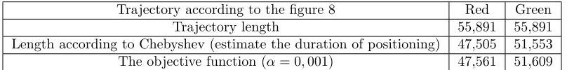
Table 1. Trajectory optimization results.

Trajectory according to the figure 8 Red Green

Trajectory length 55,891 55,891

Length according to Chebyshev (estimate the duration of positioning) 47,505 51,553

The objective function (α= 0,001) 47,561 51,609

Acknowledgements

This work was supported by the Russian Science Foundation, the agreement number 16-19-00148.

References

[1] J. Cort´es and T. Sim´eon. Probabilistic motion planning for parallel mechanisms. In IEEE Int. Conf. on Robotics and Automation, Taipei, September, 14-19 (2003) 4354–4359.

[2] F.A. Doronin. Kinematics of planar manipulator of parallel structure with three de-grees of freedom in Mathcad environment. Electronic journal. 1 (29) (2016) 6–20, http://tmm.spbstu.ru/29/doronin 29.pdf.

[3] K.G. Erastova and P.A. Laryushkin. Research of the working area and special positions of the flat 3-RPR manipulator in the MATLAB environment. The engineering bulletin. Electronic scientific and technical journal of Bauman MSTU, 7 (2016) 1–7.

[4] Y.G. Evtushenko, M.A. Posypkin, L.A. Rybak, and A.V. Turkin. Finding sets of solutions to systems of nonlinear inequalities, Comput. Math. and Math. Phys. 57(8) (2017) 1241–1247. https://doi.org/10.1134/S0965542517080073.

[5] Y.G. Evtushenko, M.A. Posypkin, L.A. Rybak, and A.V. Turkin. Approximating a solution set of nonlinear inequalities, Journal of Global Optimization, 71(1) (2018),129–145.

[6] M. Gallant and C. Gosselin. Singularities of a planar 3-RPR parallel manipulator with joint clearance. Robotica, 36(7), 1098–1109. doi:10.1017/S0263574718000279.

[7] M. H. Kakhki and S. Ebrahimi. Study on the Effect of Axial Forces on Dynamic Stiffening of a 3-RPR Planar Parallel Manipulator with Flexible Intermediate Links. Proceedings of the 2014 2nd RSI/MSI International Conference on Robotics and Mechatronics (ICRoM 2014) October 15-17, 2014, Tehran, Iran.

[8] S.Y. Khalapyan, L.A. Rybak, A.I. Glushchenko, and Y.A. Mamaev. On neural network model development to solve parallel robots kinematics and control problems. International Journal of Pharmacy & Technology. 8(4) (2016) 25085–25095.

[9] S.Y. Khalapyan, L.A. Rybak, and D.I. Malyshev. Determination of necessary geometric pa-rameters of tripod robot workspace, taking into account zones of singularity. Advances in Engineering Research. 133 (2017) 648–653.

[10] M.S. Korytov. Automating the design of optimal trajectories of moving cargoes mobile cranes organized in a non-uniform three-dimensional space. Omsk: Siberian State Automobile and Highway Academy (SibADI) (2012) 380 p.

transporttechnological systems: materials of the International Scientific and Technical Conference. -Tyumen: TyumGNGU, (2011) 317–322.

[12] P.A. Laryushkin and D.S. Epanchintseva. The coupling equations and the solution of the inverse positional problem for plane mechanisms of a parallel structure of arbitrary geometry. The engineering bulletin. Electronic scientific and technical journal of Bauman MSTU, 9 (2015) 12–21.

[13] M. Posypkin and A. Usov. Implementation and Verification of Global Optimization Bench-mark Problems. Open Eng., 7:1 (2017), 470–478.

[14] L.A. Rybak, S.Y. Khalapyan, and E.V. Gaponenko. Issues of planning trajectory of parallel robots taking into account zones of singularity. IOP Conf. Series: Materials Science and Engineering. 327 (2018) 042092. 1–8.

[15] Sureyya Sahin. Position Equations of a 3RPR Planar Manipulator. arXiv:1508.01733v1 [cs.RO] 7 Aug 2015. https://arxiv.org/pdf/1508.01733.pdf. pp. 1-5.

[16] J.C. Trinkle and R.J. Milgram. Complete path planning for closed kinematic chains with spherical joints. Int. J. of Robotics Research, 21(9), September (2002) 773–789.

[17] D. Xie and N.M Anamato. A kinematics-based probabilistic roadmap method for high dof closed chain systems. In IEEE Int. Conf. on Robotics and Automation, New Orleans, April (2004) 473–478.

[18] J. H. Yakey, S. M. LaValle, and L. E. Kavraki. Randomized path planning for linkages with closed kinematic chains. In IEEE Trans. on Robotics and Automation, 17(6): December (2001) 951–958.