Volume 16, Number 3, 2009 © Mary Ann Liebert, Inc. Pp. 407–426
DOI: 10.1089/cmb.2008.0081
Analysis of Gene Sets Based on the Underlying
Regulatory Network
ALI SHOJAIE and GEORGE MICHAILIDIS
ABSTRACT
Networks are often used to represent the interactions among genes and proteins. These
interactions are known to play an important role in vital cell functions and should be
included in the analysis of genes that are differentially expressed. Methods of gene set
analysis take advantage of external biological information and analyze
a priori
defined sets
of genes. These methods can potentially preserve the correlation among genes; however,
they do not directly incorporate the information about the gene network. In this paper,
we propose a latent variable model that directly incorporates the network information. We
then use the theory of mixed linear models to present a general inference framework for
the problem of testing the significance of subnetworks. Several possible test procedures are
introduced and a network based method for testing the changes in expression levels of
genes as well as the structure of the network is presented. The performance of the proposed
method is compared with methods of gene set analysis using both simulation studies, as
well as real data on genes related to the galactose utilization pathway in yeast.
Key words:
gene networks, gene set analysis, latent variable model, mixed linear model.
1. INTRODUCTION
I
N STANDARD ANALYSIS OF DIFFERENTIAL EXPRESSION, statistical significance of each gene is assessed independently, and some method of multiple testing correction is then used to adjust the estimatedp-values. Such methods are usually less sensitive in detecting genes that have smaller differences in mRNA abundance between different experimental conditions and may therefore be less powerful than desired. Furthermore, analyzing individual genes (single-gene analysis) often generates results that are not reproducible and lack meaningful biological interpretations. The focus of current research has thus shifted to analyzing a priori defined sets of genes (gene set analysis) and using external information to strengthen the analysis of differential expression. Analysis of gene sets results in increased power compared to single gene analysis. Furthermore, methods of gene set analysis can preserve the correlation among genes which may lead to more reliable inference. These methods however, do not directly incorporate the external information about the interactions among genes represented by the gene network. In this paper, we develop a model that directly incorporates the network information, and propose a general inference framework for testing the significance of genetic pathways.Department of Statistics, University of Michigan, Ann Arbor, Michigan.
1.1. A motivating example
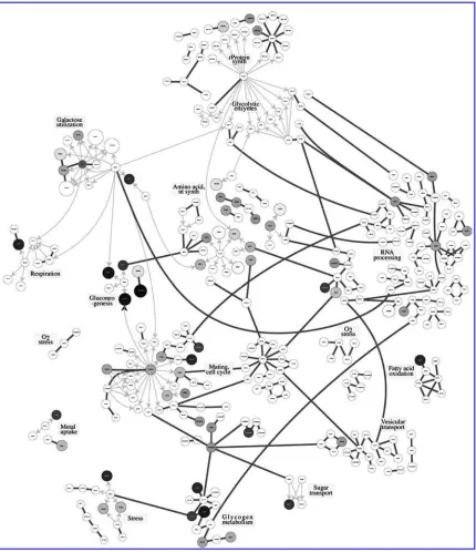
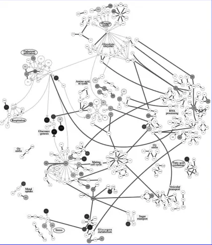
[image:2.612.73.503.181.679.2]In an interesting approach, Ideker et al. (2001) integrated gene expression and protein level data to study significant signaling and metabolic pathways in yeastSaccharomyces cerevisiae. They reported interactions among genes and proteins in different pathways along with information on the estimated correlation among genes in the network. The authors also grouped the genes into subnetworks (pathways) based on their biological functions. Figure 1, which was originally presented in Ideker et al. (2001), illustrates the network of genes under consideration. We also update the network of Ideker et al. (2001) based on newly
TABLE1. ANALYSIS OFIDEKER2001DATAUSINGGSEA
Pathway Size
NOM
p-val
FDR
q-val
FWER
p-val
Involved in gal (C= )
Galactose utilization 12 0.0020 0.00114 0.003 C Amino acid synthesis 30 0.1853 0.21562 0.676 C rProtein synthesis 28 0.5261 0.44938 0.972 C
Stress 12 0.02004 0.19283 0.108
Vesicular transport 19 0.07243 0.54138 0.489 Glycogen metabolism 12 0.1321 0.41115 0.538
Respiration 9 0.1878 0.39508 0.637
O2 stress 13 0.2384 0.6601 0.906
Fatty acid oxidation 7 0.4694 0.82373 0.963 Mating, cell cycle 58 0.3583 0.71842 0.968
Sugar transport 2 0.7358 1 0.993
Metal uptake 4 0.8374 1 0.997
Gluconeogenesis 7 0.8455 0.98853 0.997
RNA processing 75 0.9879 1 1
Glycolytic enzymes 16 0.9683 0.98189 1
The first two columns illustrate the pathway considered and the number of genes in the pathway. For each gene set, the Nominalp-value, FDRq-value, and FWERp-value are reported along with the involvement of the pathway in galC/gal conditions.
defined interactions among genes reported in Bader et al. (2004). This results in a network of 343 genes with 419 interactions for which estimates of correlations among genes are also available (this data is referred to as theIdeker datahenceforth).
The mRNA expression levels of genes in the Ideker data are measured in 9 different perturbations of GAL genes along with the wild type yeast. For each perturbation, two samples of data are available. The first set of samples represents the expression levels of genes in cells grown in presence of galactose (galC), while the second set includes expression levels for cells grown in absence of galactose (gal ), where the main source of carbon is raffinose. Our primary goal is to determine the pathways that areinvolved(either induced or suppressed) in cell growth in galCcompared to gal environments. In other words, we would like to test whether each of 15 gene sets defined by yeast pathways in the network of Ideker et al. (2001) is differentially expressed in galCcompared to gal medium.
In this section, we analyze the Ideker data using methods of gene set analysis. More specifically, we apply theGene Set Enrichment Analysis(GSEA) method of Subramanian et al. (2005). This method uses a permutation-based test (permuting the class labels) to determine whether genes ina prioridefined gene sets have non-random associations with the phenotype. To that end, we first normalize the data so that the expression levels only represent the effect of the growth environment.1 The results of the analysis are displayed in Table 1.
The first line of the table presents an expected outcome; the expression levels of genes in the Galac-tose Utilization pathway is expected to change in response to perturbations of GAL genes in the galC environment. On the other hand, although some of the pathways seem to have differential expression when cells lack galactose (e.g., Stress and Vesicular Transport), no other pathway appears significant after adjusting for multiple testing using the False Discovery Rate (FDR) controlling procedure of Benjamini and Hochberg (1995) with aq-value of 0.05. In Section 5, we revisit the analysis of the Ideker data based on the method proposed in this paper, which directly incorporates the network information represented by the gene network in Figure 1.
1The mean expression levels of the two samples corresponding to each perturbation is subtracted from the two
1.2. Background
Recent research on gene set analysis can be broadly classified into permutation-based methods motivated by the GSEA paper and model-based approaches that make specific distributional assumptions about the gene expression data. The literature can be further categorized on whether direct or indirect external information on the gene network is employed. Tian et al. (2005) considered the problem of gene set analysis and described two hypotheses that should be considered when studying the significance of sets of genes. One of these hypotheses, which is the same as the hypothesis considered in GSEA, focuses on non-random association of genes in the gene set with the phenotype. The other hypothesis, considers non-random correlations between genes in a gene set. The test method proposed for the first hypothesis is based on permuting the class labels (column permutation) and the second hypothesis is tested by permuting genes (row permutation). Efron and Tibshirani (2007) formalized the idea of gene set analysis in a coherent statistical framework and examined the hypotheses presented in Tian et al. (2005). They also proposed an alternative test statistic with superior power properties and analyzed the effects of row and column permutations. Goeman and Bühlmann (2007) reviewed different methods proposed for testing significance of gene sets and highlighted important issues in selecting appropriate methods.
Although the above permutation-based methods are computationally intensive, they include minimum assumptions about the underlying biological model and are therefore more robust to model misspecification. An alternative approach is based on model-based tests procedures, where specific distributions for the expression data are assumed. In one such approach, Jiang and Gentleman (2007) extended the idea of gene set analysis by adapting a linear model approach and adjusting for other covariates. They presented the gene sets in the form of an index matrix and offered a heuristic argument for using a normal approximation for testing per gene set sums. One major difficulty regarding model-based methods is the large number of variables (genes) compared to the small number of samples—the large p, small n problem (West, 2000). In such situations, estimation of model parameters becomes a challenging task and may result in unstable outcomes. However, additional sources of information besides the expression levels of genes could be used to make the estimation more accurate. One such source of external information is the underlying relationship between genes which itself is of independent interest. It is known that genes interact with each other through their protein products and form gene regulatory networks. Also, the protein products of groups of genes are involved in controlling specific functions in cells through genetic pathways. Increasing amount of information about these relationships is becoming available in public repositories, like the KEGG (Kyoto Encyclopedia of Genes and Genomes) (Kanehisa and Goto, 2000) and the Gene Ontology (GO) (Ashburner et al., 2000), and can be used to improve the estimates of model parameters.
A number of researchers have recently used external information about gene networks to improve the analysis of gene sets. Rahnenführer et al. (2004) demonstrated that the sensitivity of detecting relevant pathways can be improved by integrating information about pathway topology. Barry et al. (2005) presented a permutation based procedure, called SAFE, that considers the underlying network structure. More recently, Wei and Li (2007) have proposed a Markov random field model to incorporate the information on the gene network in the analysis. In a related approach, Wei and Pan (2008) have modeled the network information via latent variables into a spatially correlated mixture model. Both of these methods, consider the problem of analysis ofsingle geneson the network.
The above methods either assume that the underlying network does not change as the experimental conditions change or they do not incorporate this change directly into the model. However, changes in the underlying network structure can amplify the change in expression patterns and should be included in the analysis. For instance, Li (2002) demonstrated that the correlation patterns among ARG2 and other members of the urea-cycle pathway can change drastically as the expression level of ARG2 changes. Another concern in analyzing network data is to decorrelate subnetworks from the effects of other nodes in the network and to deal with nodes that belong to multiple networks. Alexa et al. (2006) present one such method which is an attempt to decorrelate GO graph structures. Their method focuses on decorrelating nodes at lower levels (children) from upper level nodes (parents).
the change in the expression levels of the genes in different conditions, but also reflects the change in network structures and correlations among genes. We also present a systematic approach that decorelates each subnetwork from the other nodes while maintaining the interactions among genes in the subnetwork. The rest of the paper is organized as follows. In the next section, the proposed latent variable model is introduced and some basic graph theoretical properties related to this model are discussed. In Section 3, we represent the latent variable model using the framework of mixed linear models and propose a general testing scheme based on the theory of mixed linear models. Section 3 ends with a result that is used to test the pure effect of each subnetwork. This result prevents tests of significance of subnetworks to be confounded with the effects of other subnetworks and also allows testing the effect of genes that belong to multiple networks. Section 4 includes three simulation studies for evaluating the performance of the new model under different testing conditions as well as studying the effect of noise in the network information on the proposed inference procedure. In Section 5, we revisit the Ideker data, introduced in Section 1.1, and test the significance of pathways using the proposed model. Section 6 includes a discussion on limitations of the proposed model and future extensions.
2. THE LATENT VARIABLE MODEL
Consider gene expression data Dorganized as apn matrix comprised of the expression levels ofp
genes fornsamples, and let Y be thekth sample in the expression data (kth column ofD).
To model the correlation structure caused by the gene network, we represent the network as a directed graphG D .V; E/ with vertex set V, and edge set E, where E is represented by the pp adjacency matrixA. Each nonzero element of the adjacency matrix,Aij, represents a directed edge in the network.
Elements of the adjacency matrix correspond to the strength of association among genes in the graph and are real values in. 1; 1/.
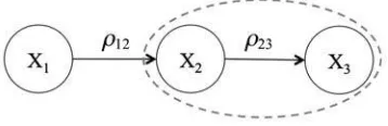
Consider the simple network of Figure 2: Suppose Y D X C", where X represents the signal and
"Np.0; "2Ip/thenoise. Consider two adjacent genes i andj, wherei affects j. One can represent
the relationship between i and j using a simple linear model Xj D ijXi. However, to account for
unknown associations among genes and/or errors in the association weights,ij, we also addlatent variables
j Np.j; 2/ to represent the baseline expression level of gene j. For instance, 2 represents the
expression level of gene 2 without the effect from gene 1. Thus, for the simple gene network of Figure 2, we obtain
FIG. 2. A simple gene network.
X1 D1
X2 D12X1C2D121C2
X3 D23X2C3D23121C232C3
These equations can be summarized in vector notation as:
Y DƒC"; Np.; 2Ip/; "Np.0; "2Ip/ (1)
whereƒis called theinfluence matrixof the graph. In the simple example above, we have
ƒD
0
B B @
1 0 0
12 1 0
1223 23 1 1
Under such a model, Y is a normal random variable with mean EŒY D ƒ and variance Var.Yi/D
2
ƒƒ0C"2Ip, whereƒ0 denotes the transpose of matrixƒ.
In the remainder of this section, we study the relationship between the influence matrix, ƒ, and the adjacency matrix of the graph,A. We provide a general result for the relationship betweenƒ andA as well as a compact expression that can be used to efficiently evaluateƒfor specific classes of graphs. We also discuss conditions under which the matrixƒhas full rank, which will be used in the analysis of the proposed inference procedure in Section 3.
Lemma 2.1. For any graphG D .V; A/ we haveƒDA0CA1CA2C DP1
rD0Ar (hereA0 is
defined to be the identity matrix).
Proof. From the matrix representation of the latent variable model in (1)
Yi D p X
jD0
ƒijj C"i; iD1; : : : ; p
whereƒi i D1 andƒij ¤0 only if there is a path (of some length) on the graph from nodeito nodej.
But for any graphG, the number of paths of lengthr (r2N) fromvi tovj is given by the.i; j /element ofAr (Diestel, 2006). Therefore,ƒij ¤0whenever there existsrsuch thatŒArij > 0. Hence, all possible
paths fromi toj are given byŒP1
rD0Arij. This implies thatƒDP1rD0Ar.
Corollary 2.2. For any Directed Acyclic Graph (DAG),ƒDA0CA1CA2C CAp.
Proof. This follows immediately from Lemma 2.1 by noting that since there are no loops in DAGs, the maximum length of paths equalsp.
The following results provide sufficient conditions for the matrix ƒ to be of full rank. Although this guarantees validity of the model for at least some classes of directed graphs, it does not provide a necessary condition. Based on experiments with randomly generated adjacency matrices, there are in fact larger classes of graphs satisfying this property.
Lemma 2.3. For any Directed Acyclic Graph (DAG), the matrixƒhas full rank.
Proof. The full rankness ofƒis proved by showing thatƒcan be re-arranged into a lower triangular matrix with 1’s on the diagonal.
First observe thatƒij ƒj iD0, since otherwise there will be a cycle in the graph. Also, from 2.1 we
haveƒi i D1.
Consider a reordering of rows (and correspondingly of columns) of the matrix in decreasing number of zeros. Every DAG has at least one root (a node that is not affected by any other node). This means that there is at least one row withƒkk D1andƒkj D0for allj. Permuteƒso that rowk is the first row of
the matrix and continue in the same way. Denote the number of zero elements of rowi byi and number
of zeros in columnj asCj. Then by the above observation,Ri p C i (herep C i is the number
of nonzero elements in columni).
To complete the proof, we need to show that the rearranged matrixƒcan be further permuted to result in a lower diagonal matrix. Suppose there exists j > i such that ƒij > 0 and therefore ƒj i D 0. If
Rj D Ri switchi andj to get a lower triangular matrix. However, ifRj < Ri (i.e., ifi is affected
by a row with less number of zeros) there existsl such that ƒj l > 0 but ƒi l D 0. However, ƒj l > 0
means there exists a path fromltoj andƒij > 0means that there exists a path fromj toi. Thus there
exists a path fromltoi, i.e.ƒi l > 0, a contradiction. Thereforeƒmust be a lower triangular matrix with
Lemma 2.4. Consider a graph G = (V,A) with influence matrixƒ
a) If G is a Directed Acyclic Graph (DAG), thenADI ƒ 1.
b) If the sum of absolute values of weights of edges ending at every node of the graphG is less than 1 (i.e.Ais sub-stochastic), thenADI ƒ 1 andƒhas full rank.
Proof. a) From Corollary 2.2, ƒDPprD0Ar and hence
AƒD
p X
rD0
ArC1DƒCApC1 I
But whenG is a DAG,ApC1D0 henceAƒDƒ I. By full rankness ofƒ,ADI ƒ 1.
b) The condition in (b) implies that the sum of the absolute values of off-diagonal elements ofAis less than 1. Letsi be the sum of absolute values of off-diagonal elements of theith row ofA. Since the diagonal
elements ofAare 0, by the Gershgorin’s Ring Theorem (Friedberg et al., 1996) ifis an eigenvalue of
A, we havejj si 1. Now letƒmDPmrD0Ar. Then ƒDlimm!1ƒm and using an argument similar
to part (a),
AƒmDƒm I CAmC1
Since eigenvalues ofA are less than 1 in magnitude, limm!1ƒm exists (Friedberg et al., 1996) and by
the eigen-decomposition ofA,AmC1!0asm! 1. Hence, taking the limit, we getAƒDƒ ICA. On the other hand, the established bound on the eigenvalues ofAimplies that all eigenvalues ofI Aare nonzero, which means thatI Aand therefore,ƒare full rank. ThusADI ƒ 1.
Lemma 2.4 establishes an alternative relationship between ƒ and A and determines two classes of graphs for which such a relationship is valid. As noted before, conditions presented in this result are only sufficient. For the general graphG D .V; A/, if the spectral radius of Ais less than 1, ƒhas full rank and the relationship between A and ƒ established in Lemma 2.4 holds. On the other hand, in special cases whereƒis not of full rank, it may be possible to modify the graph and therefore apply the model presented here. For instance, one large class of graphs whereƒis not full rank consists ofcyclicgraphs. The cycles in biological networks are often representatives of feedback loops which are common features of cell cycle related networks. However, the feedback is usually effective after a time delay and therefore, when time series data is used to study these networks, the cycles can be broken down by distinguishing between nodes at the beginning and end of each cycle. Undirected edges (e.g., protein-protein interactions) can also be transformed into two directed edges using a common latent variable affecting both nodes. More generally, it is often possible to transform the graph by introducing dummy nodes and can hence apply the model presented here.
3. INFERENCE
3.1. Preliminaries
In this section, we study the inference procedure for the proposed model. Although this method can be used to test a variety of hypotheses, in order to simplify the presentation, we focus on testing the equality of means of two experimental conditions. The extension to more complicated settings is discussed at the end of the section. As before, let Y be a given sample in the expression data (kth column of data matrix D) and let YC and YT represent control and treatment conditions, with n1 columns of D
corresponding to control samples and n2 D .n n1/ columns to treatment samples. Also let two sets
of parameters .C; ƒC/ and.T; ƒT/represent mean vectors and influence matrices under control and
treatment conditions, respectively.
Let b be an indicator vector determining genes that belong to a specific gene set (pathway). In other words,bj D1 if genej is in gene set and 0 otherwise. We can test the significance of the gene sets by
defining the test statisticVDbYT bYC and testing:
Then underH0:
E0ŒVD0
and
Var0.V/D.1=n2/Œn2.bƒT/.bƒT/0Cn1.bƒC/.bƒC/0
Although the hypothesis in (2) can be tested using a generalized likelihood ratio test, it turns out that the latent variable model of Section 2 can be represented as a Mixed Linear Model (MLM). Using this framework, we can study a variety of spatio-temporal models and consider more general hypothesis testing problems.
3.2. Mixed linear model representation
Let Y, and" represent the rearrangement of vectors Y,, and "intonp1 column vectors. Then
YD‰ˇC…C"where:
ˇD.C1; : : : ; Cp; T1; : : : ; Tp/0
‰ D ƒ
C ƒC 0 0
0 0 ƒT ƒT
!0
…Ddiag.ƒC; : : : ; ƒC; ƒT; : : : ; ƒT/0
In this model,is the vector of (unknown)random effectsandand"are normally distributed random vectors with:
E "
"
# D
"
0
0
#
and
Var
"
"
# D
"
† 0
0 †" #
For the latent variable model presented in the previous section,† D2I and†"D"2I and the variance
ofYj; j 2 fC; Tgis given by2
ƒj.ƒj/
0
C2 "I.
The estimate ofˇ in the mixed linear model is given by (Searle, 1971): O
ˇD.‰0WO 1‰/ 1‰0WO 1Y
WD.2 ……
0
C2
"Inp/. The estimate of ˇ depends on estimates of2 and"2 which can be estimated
viaRestricted Maximum Likelihoodprocedure (REML).
The framework of mixed linear models allows us to test a variety of hypotheses aboutˇby considering tests of the form:
H0WlˇD0 vs. H1 Wlˇ¤0 (3)
Herelis in general anyestimablelinear combination ofˇ’s (Searle, 1971). An example of such a vector is acontrast vector, which satisfies the constraint10lD0. In the ensuing discussion, any linear combination ofˇ’s satisfying the estimability requirement is referred to as acontrast vector.
Based on the theory of mixed linear models, we can test (3) using the test statistic:
T D l
O
ˇ
p
lC lO 0 (4)
Under the null hypothesis in (3),T has approximately at distribution withdegrees of freedom, where the degrees of freedom is estimated using the Satterthwaite approximation method (McLean and Sanders, 1988):
D 2.lC lO
0/2
0K
with D.@@2 lC l
0; @ @2
"lC l
0/0 andK is the empirical covariance matrix of.2 ; "2/0.
3.3. Computational issues and the use of the mixed linear model
The mixed linear model facilitates the representation of the latent variable introduced in Section 2. However, estimation and inference in this framework involves forming the matrices ‰ and …, and performing operations involving products and inverses of these matrices. In the context of analysis of genetic data, the dimensions of these matrices (np2p and npnp) can cause serious difficulties in terms of computation time, memory requirement and numerical stability of the estimation algorithms. It is therefore necessary to derive alternative methods for estimation of parameters in the model. It turns out that due to the special structure of the model presented in Section 2, and the sparsity pattern of matrices ‰ and…, the formulas presented in the previous section can be substantially simplified. More specifically, for the problem stated in Section 3.2 we have:
O ˇD O ˇC O ˇT ! D N YC N YT ! and C D 2 6 6 6 4 1 n1
.2IpC"2.ƒC
0
ƒC// 0
0 1
n2
.2IpC"2.ƒT
0 ƒT//
3
7 7 7 5
In the particular case considered here, the REML estimates of the variance components can be directly computed as the maximizers of the REML equation without any need for iterative methods. However, profiling out one of the variance components may result in more stable solutions.
3.4. Role of the contrast vector
The estimates ofˇ based on the mixed linear model represent the individual expression level of each gene in the network. Thus, in order to evaluate the combined effect of each gene set using the test statistic
T, the choice of contrast vectorl proves fairly crucial. More specifically, the choice ofl determines the null and alternative hypotheses of the test in (3), which in turn affects its significance level and power. In this section, we present different choices of contrast vectors and study their properties and effects on the power of tests.
A simple choice for the contrast vectorl is to use the indicator vector of the gene set. In other words,
l.1/D. b;b/ (5)
This simple choice ofl corresponds to testing the following hypothesis:
H0.1/Wb.T C/D0 vs. H1.1/Wb.T C/¤0 (6)
which for each gene setg is equivalent to
H0.1/WX i2g
Ti Ci D0 vs. H1.1/WX i2g
Such a contrast vector however, only considers the mean expression levels of genes and does not reflect the combined effect of the set of genes inb, which is affected by interactions among genes in the network. When the underlying network structure and therefore the correlation among genes is known, a natural alternative tol.1/is to also include the influence matricesƒC andƒT. This leads to the following choice of contrast vector:
l.2/D. bƒC;bƒT/ (8)
which corresponds to testing the following hypotheses:
H0.2/Wb.ƒTT ƒCC/D0 vs. H1.2/Wb.ƒTT ƒCC/¤0 (9)
The null hypothesis presented in (9) may first seem less intuitive and the choice ofl.2/ rather arbitrary.
However, the rationale behind the latter choice of contrast vector becomes clearer when we examine the test statistics corresponding to each one of the two null hypotheses in (6) and (9). In the case of the two-population test considered here, the above choices of contrast vectors lead to (after some algebra) the following test statistics:
T1D
b..ƒT/ 1YNT .ƒC/ 1YNC/ s O 2 1 n1 C 1 n2
bb0C O2 " b 1 n2
.ƒT0ƒT/ 1C 1
n1
.ƒC0ƒC/ 1
b0
(10)
and
T2D
b.YNT YNC/ s O 2 b 1 n2
ƒTƒT0C 1
n1
ƒCƒC0
b0
C O2
" 1 n1 C 1 n2 bb0 (11)
From the above two equations it becomes clear than choosingl.2/as the contrast vector leads to a very
familiar test statistic. The numerator of test statisticT2 considers the difference in average observed values
of expression levels and its denominator represents the variance ofYNT YNC based on the mixed linear
model.
It is also important to study the effect of the contrast vector on the power of tests. The two null hypotheses presented in (6) and (9) are different and therefore the usual power analysis cannot be applied to choose the right test. However, when ƒC D ƒT D ƒ, the hypothesis presented in (6) is a special case of (9)
(assuming thatƒ has full rank) and it is possible to compare the powers of the two tests in this special case. WhenƒC DƒT Dƒ, the null and alternative hypotheses are given in (6) and the test statistics T
1
andT2 have the following simplified forms:
T1D
b.ƒ 1.YNT YNC// s b 1 n1 C 1 n2
.O2
IC O"2.ƒ0ƒ/ 1/b0
(12)
T2D
b.YNT YNC/ s b 1 n1 C 1 n2
.O2
.ƒƒ0/C O"2I /b0
(13)
From these equations we can see that when no underlying network structure is taken into account, (ƒDI) the two test statistics are the same. However, if there is an underlying network structure (ƒ¤I), the test statistic in (13) represents the likelihood ratio test for testing the null hypothesis in (6), which is asymptotically most powerful. On the other hand, askƒT ƒCkincreases, the test presented byl.1/ will
no longer be appropriate and we could expectl.2/to have a better performance.
In the more general case, whereƒC ¤ƒT, it is desirable for the test statistic to account for all of the
FIG. 3. Illustration of the Network contrast vector on a simple network; dashed line indicates the interactions that are included in the contrast vector.
subnetwork. Consider again the simple gene network in Figure 2 and letbD.0; 1; 1/. It is then desirable for the test statistic to include the interaction between genes 2 and 3, while excluding the effect of gene 1 (Fig. 3). The following result describes a choice of a contrast vector that achieves this goal.
Lemma 3.1. Consider a1p indicator vector band letxy represent the element-wise product of
xandy.
Then.bƒb/ includes the effects of all the nodes inbon each other, but it is not affected by any node outside of the set of nodes indexed byb.
Proof. Let IbD fi Wbi D1g. Based on the latent variable model, thejth column ofƒ includes the
influences of nodej on all other nodes in the network. Therefore,.bƒ/j is the influence of thejth node
on all nodes inb. Also, note thatƒi i D1for alliandƒj iis non-zero only if there is a path fromj toi.
Thus,
.bƒ/j D 8 ˆ ˆ ˆ ˆ <
ˆ ˆ ˆ ˆ :
X
i2Ib
ƒj i j …Ib
1C X
i2Ib;i¤j
ƒj i j 2Ib
But.bƒb/j is non-zero only ifj 2Iband therefore
.bƒb/D X
j2Ib
jC X
j2Ib X
i2Ib;i¤j
ƒj ij
which means that.bƒb/ only includes the effects of elements ofb on each other.
The estimated ˇ’s in the latent variable model reflect the individual effect of each gene and therefore, can be thought of as the “pure signals.” Based on Lemma 3.1, in order to include interactions among genes in each subnetwork and prevent any confounding effects, we define thenetwork contrast vectorby
l.N /D. bbƒC;bbƒT/
3.5. Comparison with other gene set analysis techniques
In this section, we discuss the main differences between the approach proposed in this paper and the idea of gene set enrichment analysis (GSEA) presented in Subramanian et al. (2005) and generalized by Efron and Tibshirani (2007).
Alternatively, if efficient estimation of the covariance matrix is possible, parametric test statistics may be used to test the difference between the expression levels of the two treatment groups. This is not usually possible since in most microarray analysis applications the number of parameters needed to be estimated is considerably larger than the number of samples available (np). However, the external information about the underlying gene network can make this estimation problem tractable. For instance, in the mixed linear model proposed in this paper, the covariance matrix is modeled as a function of few parameters which can be efficiently estimated from the data. Thus, it is possible to test the significance of each gene set using tests that include the expression levels ofallgenes in the gene set and also directly incorporates the covariance structure of the genes in each subnetwork. An example of such a test statistic is theT2test
statistic discussed in Section 3.4, which is a version of the two-samplet-test. If the model is correctly specified, one could expect such a test statistic to be sensitive to changes in both the expression levels and also in the covariance structure. However, in the absence of external information about the network, estimation of the covariance matrix may be impractical and non-parametric methods like GSEA, may offer better inference properties.
In the next section, we carry out simulation studies to illustrate the difference between the proposed model and the GSEA method. We will also examine the effect of the choice of the contrast vector on the performance of the proposed test statistic.
4. PERFORMANCE ANALYSIS
Three sets of simulation studies are considered in this section. In the first simulation, we study different choices of contrast vectors and compare their performance with GSEA in a simple network. The second simulation study is designed to analyze the combined effect of change in mean and covariance between control and treatment conditions. In the last simulation, we evaluate the sensitivity of the proposed inference procedure to the presence of noise in the association weights. Note that in simulation studies of this section, it is assumed that the effect of the gene network is appropriately modeled using the latent variable model of Section 2 and that the the topology of the network is correctly specified.
4.1. Simulation 1: Different choices of contrast vector
In the first setting, a simple network structure consisting of an eight-level binary tree with 255 nodes is used. It is assumed that there are no interactions in the network under the control condition (ƒC DI).
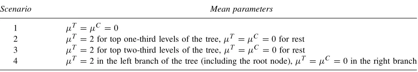
Under the treatment condition, genes on the network are assumed to be positively correlated with different association strengths: The association for the first three levels of the genes in the network (top seven genes in the tree) is assumed to be 0.8, genes in the next three levels (56 genes) have association equal to 0.5 and the remainder of the genes are weakly associated withD0:2. Under control, the mean vector for mRNA expression levels of genes is set to zero (C D 0). Scenarios for mean expression levels under treatment are presented in Table 2 and Gene sets considered in this simulation are given in Table 3. The gene sets are chosen so that for each mean scenario there exists gene sets with highly expressed genes and also gene sets that represent non-differentially expressed genes.
Table 4 presents the estimated powers of the GSEA method and tests based on the three contrast vectors,
l.1/,l.2/, andl.N /, introduced in Section 3.3 based on 1000 simulations. The powers are calculated based
on the FDR controlling procedure of Benjamini and Hochberg (1995) with aq-value of 0.05.
TABLE2. MEANSCENARIOS UNDERTREATMENT FOR THEFIRSTSIMULATIONSTUDY
Scenario Mean parameters
1 T DC D0
2 T D2for top one-third levels of the tree,T DC D0for rest 3 T D2for top two-third levels of the tree,T DC D0for rest
[image:12.612.71.501.644.718.2]TABLE3. GENESETSCONSIDERED IN THEFIRST
SIMULATIONSTUDYa
Gene set Genes considered
1 All genes in the network 2 Ttop one-third levels of the tree 3 First two-third levels of the tree 4 The last level of the tree
5 Left branch of the tree (including the root) 6 Right branch of the tree (excluding the root) 7 20% of genes in the network selected randomly
aGSEA method tests the significance of genes in the gene set against other genes not included in the gene set. We have excluded the last gene from gene set 1 to make this comparison possible, but this may not be an appropriate gene set for GSEA.
The positive correlation structure of the network affects the significance of the subnetworks selected for this comparison. When a specific gene in the network becomes differentially expressed, the other genes in the network that are influenced by that gene will also have modified expression levels in the same direction and the combined subnetwork becomes strongly significant. This propagation mechanism explains the abundance of powers of 1 in the table. The first mean scenario in this study corresponds to the case that ƒCC D ƒTT. All the methods have nominal significance level of 0.05 for this test.
On the other hand, there are some differences between the tests based on different contrast vectors and the GSEA method. As one expects from the discussion in Section 3.4, the test based onl.2/ has higher power
than the test based onl.1/. It can also be seen that in all but one case, the power resulted from test based
onl.2/ is higher than the power for the GSEA method verifying the discussion of Section 3.5. There are
few cases that deserve special attention. The GSEA method indicates no power for testing all the genes in the network under scenario 2. However, in this case the top 1/3 levels of the tree are significant and therefore it is natural to expect significant differences in overall expression levels. The same pattern can
TABLE4. RESULTS OFFIRSTSIMULATIONSTUDY
Scenario Method All Top 1/3 Top 2/3 Last level Left branch Right branch Random
1 GSEA 0.000 0.000 0.000 0.000 0.000 0.000 0.000
l.1/ 0.024 0.015 0.014 0.014 0.019 0.022 0.018
l.2/ 0.023 0.020 0.015 0.012 0.011 0.023 0.019
l.N / 0.022 0.021 0.015 0.010 0.011 0.021 0.018
2 GSEA 0.000 1.000 1.000 0.000 1.000 0.000 0.000
l.1/ 0.119 1.000 0.535 0.047 0.127 0.056 0.046
l.2/ 1.000 1.000 1.000 0.090 0.980 0.956 0.523
l.N / 1.000 1.000 1.000 0.070 0.979 0.562 0.067
3 GSEA 1.000 0.000 1.000 0.000 1.000 1.000 1.000
l.1/ 1.000 1.000 1.000 0.089 1.000 1.000 0.999
l.2/ 1.000 1.000 1.000 0.568 1.000 1.000 1.000
l.N / 1.000 1.000 1.000 0.089 1.000 1.000 1.000
4 GSEA 1.000 0.000 1.000 1.000 1.000 0.000 1.000
l.1/ 1.000 0.997 1.000 1.000 1.000 0.089 1.000
l.2/ 1.000 1.000 1.000 1.000 1.000 0.476 1.000
l.N / 1.000 1.000 1.000 1.000 1.000 0.089 1.000
Powers of tests based on GSEA and three contrast vectors for different mean scenarios. Multiple testing adjustment is based on FDR withqD0:05. Entries in italic indicate powers that are lower or higher than expected, and numbers in bold show powers
be observed when comparing the two methods for testing the right branch of the tree under the second scenario and the top 1/3 of genes under the third scenario. On the other hand, the test based on l.2/
has a high false positive rate for testing the right branch of the tree in the situation where only the left branch is up-regulated (scenario 4), while the GSEA method correctly shows no deviation from the null hypothesis. The same phenomenon can be seen for the results of testing the last level of the tree in the case where the top 2/3 levels of the tree are significant. The test based onl.2/ is not able to isolate the significance of the genes under consideration from the effect of other genes in the network and can therefore result in high false positive rates. As expected based on Lemma 3.1, the test based onl.N / resolves these shortcomings. The power of this test is close to the nominal significance level for testing the above two cases while it offers a high power in cases where the GSEA method fails to distinguish the significance of the subnetworks.
4.2. Simulation 2: Simultaneous changes in mean & covariance
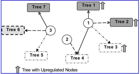
The second simulation study is designed to evaluate simultaneous changes in expressions levels as well as associations among genes. The network structure in this simulation consists of three root nodes and seven five-level trees (220 genes total). The network consists of low and high association subnetworks and also includes both positive and negative correlations. Three of the subnetworks are considered to be differentially expressed (the level of expression increases in increments of 0.2) and the other subnetworks have equal values of mean in treatment and control conditions. Figure 4 illustrates the setting of parameters of this simulation study.
Table 5 presents the estimates of powers for the GSEA method and the test based on l.N / for testing different trees with increasing expression levels in a simulation with 1000 repetitions. It can be seen from the results that both of these methods reject the null hypothesis for tests related to trees with high positive correlation (subtrees 1, 2, and 7 in Fig. 4). The GSEA method can only detect the significance of subtree 3 for large values of increase in the expression level while the test based onl.N /, can detect this change for smaller values of increase. Subtrees 4 and 5 correspond to cases where the correlation among genes is minimal. Subtree 4 is affected by root genes 1 and 2 that are both up regulated but they have opposite correlations with genes in subtree 4. As one would expect, the powers for subtree 4 are similar to those of subtree 5, which suggests that the combined effect of genes 1 and 2 on subtree 4 is the same as the effect of gene 3 on subtree 5. Subtree 6 illustrates the fact that the test based on
l.N / takes advantage of the known correlation structure even if the genes in the network are negatively
[image:14.612.149.423.521.666.2]correlated while the GSEA method cannot detect the change in the correlation structure between control and treatment conditions.
TABLE5. RESULTS OF THESECONDSIMULATIONSTUDY
Mean increase 0 0.2 0.4 0.6 0.8 1.0
Tree 1 GSEA 1.000 1.000 1.000 1.000 1.000 1.000
NetGSA 1.000 1.000 1.000 1.000 1.000 1.000
Tree 2 GSEA 1.000 1.000 1.000 1.000 1.000 1.000
NetGSA 1.000 1.000 1.000 1.000 1.000 1.000
Tree 3 GSEA 0.000 0.000 0.000 0.000 0.000 1.000
NetGSA 0.2500 0.9580 1.00 1.00 1.00 1.000
Tree 4 GSEA 0.000 0.000 0.000 0.000 0.000 0.000
NetGSA 0.263 0.277 0.298 0.278 0.298 0.295
Tree 5 GSEA 0.000 0.000 0.000 0.000 0.000 0.000
NetGSA 0.281 0.296 0.290 0.297 0.305 0.281
Tree 6 GSEA 0.000 0.000 0.000 0.000 0.000 0.000
NetGSA 0.982 0.984 0.986 0.980 0.978 0.976
Tree 7 GSEA 0.000 0.000 0.000 0.000 0.000 0.000
NetGSA 1.00 1.00 1.00 1.00 1.00 1.00
Estimated powers for the GSEA and the test based onl.N /for different mean scenarios and different subnetworks. In results for each subnetwork, the first row represents the power for the GSEA method, and the second row displays the power for the test based onl.N /. Settings of fonts and colors are similar to Table 4.
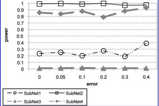
4.3. Simulation 3: Effect of noise in network information
In the last simulation, we evaluate the sensitivity of the proposed inference procedure to presence of noise in association weights of the gene network. The network consists of four similar subnetworks, each with 40 genes. Under control, genes have mean C D1 and the weights of the adjacency matrix are set
to 0.2. The settings of the parameters under treatment are given in Table 6. The estimated powers of tests of significance of each subnetwork using a test based on l.N / are plotted in Figures 5 and 6. Figure 5
represents the case where the errors are introduced at random, that is, each weight in the adjacency matrix under treatment is perturbed by a uniform noise in the range [ e; e] whereeis a value between 0 and 0.4. On the other hand, Figure 6 represents the estimated powers of tests when a systematic bias is included in the weights of the adjacency matrix under treatment. It can be seen that if the underlying model is correctly specified, presence of random noise in weights of adjacency matrix will not significantly affect the power of the test. However, presence of systematic bias in the estimated weights can introduce both type I, as well as type II errors. This is illustrated by the increase of power of the test as the difference between weights under treatment and control becomes more significant (Fig. 6). It is important to note that the simulation considered here does not include errors in the topology of the network. These errors become more critical if the topology of the network, as well as the association weights, are estimated from expression data, which is beyond the scope of this article.
TABLE6. SIGNIFICANTPARAMETERS OF THETHIRD
SIMULATIONSTUDY UNDERTREATMENTCONDITION
Subnetwork Mean Association weight
1 T D1:5 T D0:6
2 — T D0:6
3 — —
4 T D1:5 —
FIG. 5. Estimated powers of test of significance of subnetworks of Table 6 withrandom noise in weights of the adjacency matrix. Plots in gray represent the powers of subnetworks whose true adjacency matrices in control and treatment are the same.
5. ANALYSIS OF YEAST GALACTOSE UTILIZATION PATHWAY DATA
In Section 1.1, we analyzed the yeast GAL pathway data (Ideker data) using the GSEA method, which revealed that the Galactose Utilization pathway is significantly activated in galCcondition. In that analysis, the external information provided by the network was only used to determine the gene sets of interest. As discussed in Section 1.1, the Ideker data also includes strength of gene interactions in the network. Therefore, it is possible to directly incorporate the network information and use the proposed network-based inference procedure. It is important to note that the Ideker data only includes one set of association weights for both galCand gal conditions. In other words, in this section we assume ƒT DƒC Dƒ, and hence
[image:16.612.120.454.510.679.2]the proposed inference procedure cannot test the change in the network structure. Assuming that the latent variable model correctly represents the effect of the underlying network, the increased power of the network based procedure is mainly due to directly incorporating the network information.
Table 7 compares results of analyzing the Ideker data using the GSEA method and the network based method presented in this paper (using l.N /). This table also includes results of analyzing this
TABLE7. ANALYSIS OFIDEKER2001DATAUSINGGSEA, GSA,AND THE PROPOSEDMETHOD
BASED ON THEUNDERLYINGGENE NETWORKUSING THEl.N / CONTRASTVECTOR
GSEA GSA NetGSA
Pathway Size
NOM
p-val
FDR signif
NOM
p-val
FDR signif
NOM
p-val
FDR signif
rProtein synthesis 28 0.5261 0.278 0.0038 3
Glycolytic enzymes 16 0.9683 0.357 0.2825
RNA processing 75 0.9879 0.386 0.479
Fatty acid oxidation 7 0.4694 0.299 0.0068 3
O2 stress 13 0.2384 0.285 0.4448
Mating, cell cycle 58 0.3583 0.417 0.4317
Vesicular transport 19 0.07243 0.156 0.3693
Sugar transport 2 0.7358 0.458 0.3319
Glycogen metabolism 12 0.1321 0.034 0.3057
Stress 12 0.02004 0.007 0.0000 3
Metal uptake 4 0.8374 0.326 0.0802
Respiration 9 0.1878 0.091 0.0001 3
Gluconeogenesis 7 0.8455 0.475 0.0383
Galactose utilization 12 0.002045 3 0.001 3 0.0000 3
Amino acid synthesis 30 0.1853 0.054 0.0665
For each method, the nominalp-value and whether the pathway is significant based on the FDR withqD0:05is reported.
data using the GSA method of Efron and Tibshirani (2007).2 As one may expect, all three methods find the Galactose Utilization pathway to be statistically significant. Although the GSEA and the GSA methods agree on the significance of other subnetworks, it can be seen from Table 7 and Figure 7, that including the underlying network structure in the analysis, reveals four additional significant pathways. Although additional experiments are needed to verify the result of Table 7, the biology of yeast cells may offer some insight to significance of newly detected pathways. These pathways can be categorized into two groups: Galactose Utilization and rProtein Synthesis pathways are involved in cell growth in galCenvironment, while genes in the Stress, Respiration and Fatty Acid Oxidation pathways are induced in gal environment. The Stress pathway has a low nominal p-value in both GSEA and GSA results; however, these methods do not consider this pathway significant. The significance of the Stress pathway is not surprising and can be explained by the fact that galactose is a more efficient source of carbon than raffinose. Thus, in absence of galactose (gal ), the genes in the Environmental Stress Response (ESR) are induced (Gasch et al., 2000; Gasch and Werner-Washburne, 2002). The Fatty Acid Oxidation and Respiration pathways are also upregulated in gal environment. The genes in the Respiration pathway are among the genes that are induced in the ESR.
Many of the stress defense mechanisms consume ATP, and therefore, cellular stress could lead to the induced expression of respiration genes (Hohmann and Mager, 2003). Also, many genes involved in importing and exporting fatty acids are induced in ESR and the induction of these genes can increase the local concentration of fatty acids, which in turn may induce the expression of genes in Fatty Acid Oxidation pathway (Hohmann and Mager, 2003). The induction of Fatty Acid Oxidation and Respiration genes can be further explained by the coregulation of genes in these pathways. It should be noted that two of the genes in the Respiration pathway are directly affected by genes in GAL pathway (GAL4 regulates CYC1 and HAP4 is regulated by MIG1), and our proposed model can exploit such relationship in order to gain more statistical power. Finally, the significance of the rProtein Synthesis genes can be explained by growth dependent expression of these genes and the fact that ESR represses the expression of many protein synthesis genes (Hohmann and Mager, 2003).
FIG. 7. Yeast gene network indicating the significant pathways; significant pathways have been marked with ovals.
6. DISCUSSION
incorporates the weighted adjacency matrix of the network through a latent variable model and uses a flexible mixed linear representation. We discussed that the inference based on this method depends on the choice of the contrast vector and proposed a choice that offers improvement in power of the test compared to the GSEA method of Subramanian et al. (2005). The simulation studies and the analysis of the yeast galactose utilization pathway reveal the ability of the proposed method in identifying significant pathways that are otherwise difficult to distinguish. Although the focus of this paper was on testing the significance of subnetworks in the two population inference problem, the proposed method provides a general framework for studying a variety of phenotypes including analysis of time series mRNA data and the change in the network over time. More generally, different correlation structures among observations can be implemented in the mixed linear model and therefore, different types of data can be modeled using this framework. Considering parameters for environment factors and gene-gene and gene-environment interactions is also a straight forward extension of the proposed model.
The model presented in this paper relies on two main assumptions: (a) The relationship between the expression levels of genes in the network can be represented linearly using the influence matrix of the network and (b) that the data follows a normal distribution. Although the first assumption is a crucial part of this analysis, the second assumption can be relaxed using the Generalized Mixed Linear Model (GMLM) framework. However, this would make the computational aspects of the problem more challenging.
The growth of information available on the underlying biological networks calls for effective methods that can utilize such information efficiently and requires extensions of statistical methods appropriate for studying of network structures. The model presented in this paper requires external information on the weighted adjacency matrix of the network. Although more data is becoming available on gene and protein networks, many available network data only include the binary association among genes (network topology) and do not include information about the strength or direction of associations among genes. The problem of estimating the weighted adjacency matrix of the network, which is related to estimation of the covariance matrix, is of separate interest and is beyond the scope of this paper. Chaudhuri et al. (2007) propose an efficient algorithm for estimating the association among genes when the topology of the network is known. The method proposed in this paper can also be extended to the cases where only partial information about the network is available.
ACKNOWLEDGMENTS
We would like to thank the CoEditor-in-Chief, Professor Sorin Istrail, and two anonymous referees for helpful comments and suggestions. We are also thankful to Professor Trey Ideker for providing the yeast Galactose Utilization data and helpful discussions. The work of George Michailidis was partially supported by the NIH (grant 5P 41RR018627) and the MEDC (grant GR-687).
DISCLOSURE STATEMENT
No competing financial interests exist.
REFERENCES
Alexa, A., Rahnenfuhrer, J., and Lengauer, T. 2006. Improved scoring of functional groups from gene expression data by decorrelating GO graph structure.Bioinformatics22, 1600–1607.
Ashburner, M., Ball, C., Blake, J., et al. 2000. Gene ontology: tool for the unification of biology. The Gene Ontology Consortium.Nat. Genet.25, 25–29.
Bader, J.S., Chaudhuri, A., Rothberg, J.M., et al. 2004. Gaining confidence in high-throughput protein interaction networks.Nat. Biotechnol.22, 78–85.
Benjamini, Y., and Hochberg, Y. 1995. Controlling the false discovery rate: a practical and powerful approach to multiple testing.J. R. Statist. Soc. Ser. B57, 289–300.
Chaudhuri, S., Drton, M., and Richardson, T. 2007. Estimation of a covariance matrix with zeros.Biometrika94, 199–216.
Diestel, R. 2006.Graph Theory. Springer-Verlag, New York.
Efron, B., and Tibshirani, R. 2007. On testing the significance of sets of genes.Ann. Appl. Statist.1, 107–129. Friedberg, S.H., Insel, A.J., and Spence, L.E. 1996.Linear Algebra. Prentice Hall, Englewood Cliffs, NJ.
Gasch, A.P., Spellman, P.T., Kao, C.M., et al. 2000. Genomic expression programs in the response of yeast cells to environmental changes.Mol. Biol. Cell11, 4241–4257.
Gasch, A.P., and Werner-Washburne, M. 2002. The genomics of yeast responses to environmental stress and starvation.
Funct. Integr. Genomics2, 181–192.
Goeman, J.J., and Bühlmann, P. 2007. Analyzing gene expression data in terms of gene sets: methodological issues.
Bioinformatics23, 980–987.
Hohmann, S., and Mager, W. 2003.Yeast Stress Responses. Springer, New York.
Ideker, T., Thorsson, V., Ranish, J., et al. 2001. Integrated genomic and proteomic analyses of a systematically perturbed metabolic network.Science292.
Jiang, Z., and Gentleman, R. 2007. Extensions to gene set enrichment.Bioinformatics23, 306–313.
Kanehisa, M., and Goto, S. 2000. KEGG: Kyoto Encyclopedia of Genes and Genomes.Nucleic Acids Res.28, 27–30. Li, K.-C. 2002. Genome-wide coexpression dynamics: theory and application.Proc. Natl. Acad. Sci. USA99, 16875–
16880.
McLean, R.A., and Sanders, W.L. 1988. Approximating degrees of freedom for standard errors in mixed linear models.
Proc. Statist. Comput. Sect. Am. Statist. Assoc., pgs. 50–59.
Rahnenführer, J., Domingues, F.S., Maydt, J., et al. 2004. Calculating the statistical significance of changes in pathway activity from gene expression data.Statist. Appl. Genet. Mol. Biol. 3, 16.
Searle, S.R. 1971.Linear Models. John Wiley & Sons, Inc., New York.
Subramanian, A., Tamayo, P., Mootha, V., et al. 2005. Gene set enrichment analysis: a knowledge-based approach for interpreting genome-wide expression profiles.Proc. Natl. Acad. Sci. USA102, 15545–15550.
Tian, L., Greenberg, S.A., Kong, S.W., et al. 2005. Discovering statistically significant pathways in expression profiling studies.Proc. Natl. Acad. Sci. USA102, 13544–13549.
Wei, P., and Pan, W. 2008. Incorporating gene networks into statistical tests for genomic data via a spatially correlated mixture model.Bioinformatics24, 404–411.
Wei, Z., and Li, H. 2007. A Markov random field model for network-based analysis of genomic data.Bioinformatics
23, 1537–1544.
West, M. 2000. Bayesian regression analysis in the largep smallnparadigm. Technical report. Institute of Statistics and Decision Sciences.
Address reprint requests to: Ali Shojaie Department of Statistics University of Michigan 269 West Hall 1085 South University Avenue Ann Arbor, MI 48109
1. A. Shojaie, G. Michailidis. 2010. Discovering graphical Granger causality using the truncating lasso penalty. Bioinformatics26:18, i517-i523. [CrossRef]
2. A. Shojaie, G. Michailidis. 2010. Penalized likelihood methods for estimation of sparse high-dimensional directed acyclic graphs.