A Nonlinear Model with Latent Process for Cognitive Evolution
Using Multivariate Longitudinal Data
C´ecile Proust,1,∗ H´el`ene Jacqmin-Gadda,1 Jeremy M. G. Taylor,2 Julien Ganiayre,1 and Daniel Commenges1
1INSERM E0338, Universit´e de Bordeaux 2, 146 rue L´eo Saignat, 33076 Bordeaux Cedex, France
2Department of Biostatistics, University of Michigan, 1420 Washington Heights, Ann Arbor, Michigan 48109,
U.S.A.∗email:[email protected]
Summary. Cognition is not directly measurable. It is assessed using psychometric tests, which can be viewed as quantitative measures of cognition with error. The aim of this article is to propose a model to describe the evolution in continuous time of unobserved cognition in the elderly and assess the impact of covariates directly on it. The latent cognitive process is defined using a linear mixed model including a Brownian motion and time-dependent covariates. The observed psychometric tests are considered as the results of parameterized nonlinear transformations of the latent cognitive process at discrete occasions. Estimation of the parameters contained both in the transformations and in the linear mixed model is achieved by maximizing the observed likelihood and graphical methods are performed to assess the goodness of fit of the model. The method is applied to data from PAQUID, a French prospective cohort study of ageing.
Key words: Cognitive ageing; Mixed model; Multiple outcomes; Random effects.
1. Introduction
In cognitive ageing studies, cognition is generally evaluated through a battery of psychometric tests, which are quantita-tive measures of various dimensions of cognition. Describing cognitive evolution and assessing the impact of covariates on this evolution is an interesting approach to help us understand the process of cognitive ageing. As the various psychometric tests are highly correlated, multivariate longitudinal analy-ses of several psychometric tests are often performed using multivariate linear mixed models (Hall et al., 2001; Harvey, Beckett, and Mungas, 2003; Sliwinski, Hofer, and Hall, 2003). These models highlight both the differences in the shapes of evolution for each dimension and the strong correlation be-tween the dimensions.
The idea of a latent cognitive process explaining the cogni-tive decline in the elderly is hypothesized in neuropsychology. This latent cognitive process can be viewed as a common cog-nitive factor across all the psychometric tests (Salthouse et al., 1996; Fabrigoule et al., 1998) and is supposed to be a better predictor of dementia and cognitive decline. As a consequence, it would be of substantial interest to focus the analysis on this latent process by describing its evolution and evaluating the impact of covariates directly on it.
In a cross-sectional framework, Sammel and Ryan (1996) proposed a latent variable model in which covariates could affect directly the latent variable, and the multiple out-comes were assumed to be measures of the underlying latent variable with error. In a longitudinal framework, Gray and Brookmeyer (1998) proposed a marginal regression model, with estimation via generalized estimating equations, to
assess an overall treatment effect on several continuous and re-peated outcomes. Roy and Lin (2000) also extended the linear latent variable model of Sammel and Ryan (1996) to repeated multivariate data. In practice, the assumption of a linear rela-tionship between the outcomes and a Gaussian latent variable is frequently too strong, because the psychometric tests often have non-Gaussian distributions due to different metrological properties and different behaviors with ageing (Hall et al., 2001; Amieva et al., 2005). For instance, some tests may be more sensitive to changes at high levels of cognition than at low levels of cognition, while others may have the same sen-sitivity at high and low levels of cognition. Thus, we propose to introduce parameterized flexible nonlinear transformations to link the quantitative tests with the latent process. The la-tent process is defined in continuous time by a linear mixed model including a Brownian motion, and nonlinear transfor-mations of the psychometric tests are noisy measures of the latent process at discrete occasions, the shapes of the esti-mated nonlinear transformations giving information on the metrological properties of each test.
This extension of mixed models to latent variable mod-els is related to structural equation modmod-els (SEM), mainly developed in psychometrics, because in both approaches the quantity of interest cannot be measured directly and is eval-uated instead by a set of outcomes or items (Muth´en, 2002; Dunson, 2003; Rabe-Hesketh, Skrondal, and Pickles, 2004). Thus the formulation of the model has two components, a measurement model which links the latent variables with the observations and a structural model which explains the la-tent variable structure. In the last decade, there have been
major improvements in SEM (S´anchez et al., 2005). These include (i) to handle clustered or repeated data (Longford and Muth´en, 1992; Dunson, 2003; Rabe-Haseketh et al., 2004; Skrondal and Rabe-Hesketh, 2004; Song and Lee, 2004), (ii) to allow mixture of count, ordinal, and dichotomous out-comes (Dunson, 2003; Lee and Song, 2004; Rabe-Hasketh et al., 2004), (iii) to relax linearity of the relationship be-tween the latent variables by using nonlinear structural mod-els (J¨oreskog and Yang, 1996; Arminger and Muth´en, 1998; Wall and Amemiya, 2000; Lee and Song, 2004; Song and Lee, 2004), and (iv) to relax linearity between the continuous re-sponses and the latent variables (Yalcin and Amemiya, 2001). Our modeling approach differs in a number of ways. First, we focus on the change over time of a single common latent process, while the main interest of SEM lies in the relation-ship between several latent variables. Moreover, when deal-ing with quantitative outcomes, SEM generally assumes a Gaussian or a Poisson distribution for the outcomes. Except for threshold models for ordinal data (Dunson, 2003; Lee and Song, 2004; Rabe-Hesketh et al., 2004), when nonlinear trans-formations link the latent variables and the outcomes, they do not depend on parameters to be estimated. As thresh-old models are not appropriate for quantitative scores with many possible values, we estimate the shape of the transfor-mations by using parameterized nonlinear functions. Finally, our model includes a continuous-time latent process; this gives a description of the evolution of the latent cognitive level for all times in the range of the observations and furthermore, it can easily handle data where the number and times of the observations are different for each subject and for each outcome.
Nonlinearity in SEM either in the structural model or in the relationship between observed outcomes and latent variables requires the development of suitable estimation methods. For models including products of latent variables, J¨oreskog and Yang (1996) proposed a frequentist approach based on the maximization of the likelihood, while Arminger and Muth´en (1998) proposed a Bayesian approach using a Markov chain Monte Carlo (MCMC) algorithm. For models with nonlinear relationships between the responses and the latent variables, Yalcin and Amemiya (2001) proposed to compute a quadratic approximation of the nonlinear transformations, and then maximized the approximate likelihood. In contrast, to han-dle the nonlinear relationships between the responses and the latent process, we propose to maximize the exact likelihood of the observed data, which is a product of the likelihood of the transformed data (the transformed data are multivariate Gaussian in our model) and the Jacobian of the nonlinear transformations.
The main characteristics of our methodology can be sum-marized as follows:
(a) it can be applied to multivariate longitudinal non-Gaussian quantitative outcomes;
(b) it can study the evolution of a continuous-time latent process representing the common factor across all the outcomes;
(c) it can estimate the shape of the transformations link-ing the quantitative outcomes and the underlylink-ing latent process;
(d) it can handle any type of unbalanced data (number and time of measurements, covariates,. . .) and missing at random data;
(e) it can estimate impact of covariates on both the latent process and the observed outcomes.
The next section focuses on the formulation of the model for the latent process and the outcomes on the parameterized nonlinear transformations. Section 3 is devoted to maximum likelihood estimation (MLE). In Section 4 we discuss goodness of fit and Section 5 focuses on an application of the method to data from the French prospective cohort study PAQUID (Letenneur et al., 1994).
2. Methodology
2.1 The Latent Process: Structural Model
Consider the continuous-time latent process Λi = (Λi(t))t≥0
representing the common cognitive factor for individualiwith i= 1,. . .,N. Λi is defined at time t, t∈R+ according to a
linear mixed model,
Λi(t) =X1i(t)Tβ+Zi(t)Tui+σwwi(t), t≥0, (1)
whereX1i(t) is theq1vector of time-dependent covariates
as-sociated with the vector of fixed effectsβ. The (p+ 1) vector Zi(t) = (1, t,. . .,tp)T is a time polynomial of degree p (or any vector of functions of time) and the vector of random effects at subject levelui ∼N(μ,D), whereDis an unstruc-tured positive definite matrix. The processwi = (wi(t))t≥0 is
a standard Brownian motion;wi(t) models local variation and departure from the polynomial trend while the random effects account for the variability of the trend across the subjects. No independent error is added because this latent process is as-sumed to represent the actual cognition in continuous time. Note that the linearity inβor in the covariates is not crucial. Any function of time could be included in the model, because the model is still linear in the random effects, to ensure the normality of the latent process. Moreover, the Brownian mo-tion also adds flexibility to the parametric funcmo-tion of time.
2.2 The Measurement Model
Now considerKquantitative outcomes. Each outcome could be an individual psychometric test, or the sum of scores from an itemized test. For subjectiand outcomek, we observe the
nik vector of measurements yik= (yi1k, . . . , yijk, . . . , yinikk)
T,
whereyijkis the score of subjectiat occasionjfor testk. The number and times of measurements may be completely differ-ent for each subject and each outcome. In the spirit of latdiffer-ent growth curve modeling (Muth´en, 2002) and SEM (Yalcin and Amemiya, 2001), we assume that this measurementyijkis re-lated to the latent process at timetijk through the following flexible model,
gk(yijk;ηk) = ˜yijk= Λi(tijk) +αik+X2i(tijk)Tγk+ijk, (2)
where the functiongk comes from a family of nonlinear trans-formationsGdepending on the vector of parametersηk, which will be estimated; the random effects αik are independently distributed according to anN(0, σ2
αk) distribution; the
vec-tors X2i(tijk) and γk are, respectively, a q2 vector of
for the testk;ijk are independent Gaussian errors with mean 0 and varianceσ2
k.
As in Dunson (2003), the random effectαikaccounts for the fact that for a same value of the latent process, two subjects can score differently in the cognitive domain associated with psychometric testk. The contrastsγk make the relationship between the outcomes and the latent process more flexible by allowing some covariates to be differently associated with the various outcomes. The sum of the contrasts over theK tests for a given covariate equals 0. Thus, parametersβin (1) cap-ture the mean association with the covariates contained both inX1i(t) andX2i(t), while parameters γk in (2) capture the variability of the association for each test around this mean value.
2.3 The Choice of the Family of FunctionsG
For all the outcomes, the transformationsgk(y;ηk) come from the same family of functionsG. The choice of the family is a key aspect of the model; it determines the flexibility of the link between the joint outcomes with various behaviors and the underlying latent process. The transformations must be monotonic and increasing functions ofyand depend on few parameters to make the estimation of the model easier. So, the choice of the familyGis a compromise between flexibility and parsimony.
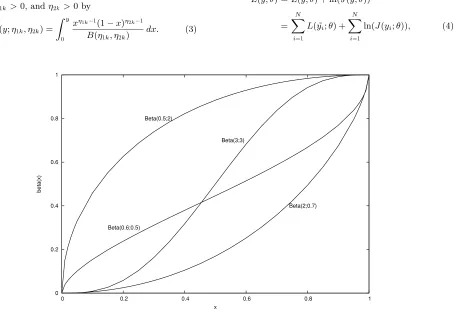
The first transformation considered here is the beta cumu-lative distribution function (CDF), which can take very differ-ent shapes, including concave, convex, and sigmoid, according to the parameters, as illustrated in Figure 1. It is defined for y∈[0, 1],η1k >0, andη2k >0 by
gk(y;η1k, η2k) = y
0
xη1k−1(1−x)η2k−1
B(η1k, η2k)
dx. (3)
0 0.2 0.4 0.6 0.8 1
0 0.2 0.4 0.6 0.8 1
beta(x)
x Beta(0.5;2)
Beta(0.6;0.5)
Beta(3;3)
[image:3.612.92.546.398.712.2]Beta(2;0.7)
Figure 1. Examples of beta transformations for various pairs of parameter values.
As the beta CDF is defined in [0, 1], for each psychometric test, a preliminary step consists of rescaling the tests to the unit interval.
The main drawback of this transformation is its computa-tional complexity. As a consequence, simpler transformations have also been considered to compare the fits of the models: the linear transformation, the logit transformation combined with a linear transformation, and the Weibull cumulative dis-tribution function (details in the Appendix). When using a linear transformation, the model is a multivariate linear mixed model similar to Roy and Lin (2000) or Rabe-Hesketh et al. (2004), with an additional Brownian motion term. In that case, constraints have to be added to make the model identi-fiable: we assume the interceptμ0equals 0 and the variance of
the random interceptu0i equals 1. In contrast, when using a CDF, the requirement thatgk(y) is in [0, 1] avoids additional constraints on the latent process.
3. Estimation
Parameter estimation is achieved using maximum likeli-hood techniques assuming that missing data are missing at random. A nonstandard aspect of the model is the pres-ence of parameters both in the nonlinear transformation
gk of the outcome and in the model for the transformed response ˜yi= (˜yi11, . . . ,y˜ini11, . . . ,y˜ijk, . . . ,y˜i1K, . . . ,y˜iniKK)
T,
where ˜yijk=gk(yijk). The log likelihood of interest is the log likelihood of the outcomes in their natural scale, and thus includes the Jacobian of the transformationsgk. It is given by
L(y;θ) =L(˜y;θ) + ln(J(y;θ))
= N
i=1
L( ˜yi;θ) + N
i=1
where θ is the complete vector of parameters containing the transformation parameters ηk = (η1k, η2k), k= 1, . . . , K, the fixed parametersμ, β, γ1, . . . , γK, and the variance–covariance parameters vec(D), σw, σα1, . . . , σαK, σe1, . . . , σeK. J(y;θ) is
the Jacobian of the transformation given the data and the vector of parameters θ. For the beta transformation, the Jacobian is defined by
J(yi;θ) = K k=1 nik j=1
yη1k−1
ijk (1−yijk)η2k−1 B(η1k, η2k)
. (5)
Formulae of the Jacobian for the other potential transfor-mations are given in the Appendix.
L( ˜yi;θ) is the log likelihood of the transformed data for sub-jecti. LetZk
i = (Z(ti1k), . . . , Z(tinikk))
T be then
ik ×(p+ 1) matrix of time polynomials for subject i and test k; Xk
1i= (X1i(ti1k), . . . , X1i(tinikk))
T and Xk
2i= (X2i(ti1k), . . . , X2i(tinikk))
T are, respectively, the n
ik × q1 matrix of
time-dependent covariates for the latent process andnik ×q2
ma-trix of time-dependent covariates for the psychometric tests. LetIn be the identity matrix of size n, andJn, the matrix of sizenwhere all the elements equal 1. Then, the density of ˜yi is a multivariate Gaussian density of sizeni=
K
k=1nik with
meanEi= (ETi1,. . .,EiKT)T and covariance matrixVigiven by
Eik =Zikμ+X1kiβ+X2kiγk (6)
Vi =
⎛ ⎜ ⎝ Z1 i .. . ZK i ⎞ ⎟ ⎠DZ1T
i · · · ZiKT
+Vw+
⎛ ⎜ ⎝
Σ1 0 0
0 . .. 0
0 0 ΣK
⎞ ⎟ ⎠,
with Σk=σ2
αkJnik+σ 2
kInik (7)
andVw the covariance matrix for the Brownian process with argumentσ2
w(min(tl,tm)) for (l,m)∈[1,ni]2. The contribu-tion of subjectito the log likelihood of the transformed data L( ˜yi;θ) is the logarithm of this multivariate density taken at the observation values. The log likelihood (4) has a closed form (except for the computation of the beta CDFs for which standard routines are available) and is maximized using a modified Marquardt algorithm (Marquardt, 1963), which is a Newton–Raphson-like algorithm. The vector of parametersθ is updated until convergence using
θ(l+1)=θ(l)−δH˜(l)−1∇Ly;θ(l). (8)
The stepδequals 1 by default but can be modified to ensure that the likelihood is improved at each iteration. The matrix
˜
H is a diagonal-inflated Hessian to ensure positive definite-ness.∇(L(y;θ(l))) is the gradient of the log likelihood (4) at
iterationl. First and second derivatives are computed by finite differences. The program is written in Fortran90 and is avail-able on the web site http://www.isped.u-bordeaux2.fr. This algorithm is less computationally demanding than al-ternative Monte Carlo approaches such as in Arminger and Muth´en (1998), who proposed a Bayesian approach for latent variable models with nonlinear relationships between the la-tent variables. Nevertheless, it is computationally intensive and, for example, with a sample of 563 subjects (8227 obser-vations) and a model with 36 parameters (the final model in
the application), the CPU time is around 15 minutes using a Bi-Xeon 3.06 GHz 1024 MB RAM.
Moreover, after convergence, standard error estimates of the parameter estimates are directly obtained using the in-verse of the Hessian. A bootstrap method using 200 resamples of theNsubjects is also performed for obtaining standard er-rors ofgk(y,ηˆk), whereyis in the range of the psychometric testk.
4. Assessment of the Fit
An unsolved question in mixed modeling is the assessment of the goodness of fit. In this work, we propose two approaches to evaluate the adequacy of the model, a residual-based ap-proach and a prediction-based apap-proach. The residual-based approach consists of evaluating the Gaussian distribution of the standardized marginal residuals ˆi given by
ˆ
i=Ui( ˜yi−Eˆi), (9)
whereUiis the upper triangular matrix of the Cholesky trans-formation ofV−1
i and ˆEi=Eθˆ(˜yi) is obtained by replacing the parameters by their MLE in (6). A normal quantile plot with the 95% confidence bands computed using the Kendall and Stuart formula (Kendall and Stuart, 1977, p. 251) is then dis-played to evaluate whether the empirical distribution of the standardized residuals ˆijk is close to the theoreticalN(0, 1) distribution.
To evaluate the fit of the data on the natural scale of the tests, we plot the observed mean evolution of each test versus the estimated marginal mean evolution or the con-ditional mean evolution, which includes random effects es-timates. The marginal estimated meansEθˆ(g−k1(˜yijk)) and the conditional estimated meansEθˆ(g−k1(˜yijk)|uˆi,αˆik,wˆi) are com-puted by numerical integration ofg−1
k (˜yik) over the marginal distribution of ˜yik, N(Eik(ˆθ);Vi(ˆθ)), or over the conditional distribution N(Eik(ˆθ) + ˆWik; ˆσkInik). Here the marginal
ex-pectation and variance of ˜yik is given by (6) and (7) and ˆ
Wijk=Zi(tijk)Tˆu
i+ ˆwi(tijk) + ˆαik is the empirical Bayes esti-mate of the subject-specific deviation from the model.
5. Application: Cognitive Evolution in the Elderly
5.1 The Data
The aim of this analysis is to describe the decline with age of the global cognitive ability measured by several psychometric tests and to evaluate the association of covariates, especially Apolipoprotein E (apoE) genotype, with the latent cognitive process. Indeed, the presence of one or two4 alleles of apoE is associated with a higher risk of Alzheimer’s disease (Farrer et al., 1997) but it is not well established whether the4 allele is more generally associated with cognitive ageing (Winnock et al., 2002).
were free of dementia at the first follow-up and with at least one measurement for each of four (K= 4) psychometric tests during the follow-up.
The four tests considered are the Mini Mental State Ex-amination (k = 1), the Isaacs Set Test (k = 2), the Benton Visual Retention Test (k = 3), and the Digit Symbol Sub-stitution Test of Wechsler (k = 4). The Mini Mental State Examination (MMSE) evaluates various dimensions of cog-nition (memory, calculation, orientation in time and space, language, and word registration); it ranges from 0 to 30 and the distribution is strongly skewed to left with a ceiling effect. The Isaacs Set Test (IST) shortened at 15 seconds evaluates verbal fluency accounting for the speed of execution: subjects have to give a list of words (with a maximum of 10 words) in four semantic categories. It ranges from 0 to 40 and the distribution is close to a Gaussian distribution with a little heavier left tail. The Benton Visual Retention Test (BVRT) evaluates visual memory: subjects have to recognize 15 geo-metric figures among four proposals. It ranges from 0 to 15 and the distribution is skewed to left but the ceiling effect is less strong than for the MMSE. The Digit Symbol Substitu-tion Test of Wechsler (DSSTW) evaluates attenSubstitu-tion: given a table of correspondence between symbols and numbers, sub-jects have to translate a sequence of 90 numbers into the right sequence of symbols. In the sample, it ranges from 0 to 76 and the distribution is approximately Gaussian. For the four tests, low values indicate a more severe impairment. In the analysis, rescaled scores computed as the value of the test plus 0.5 divided by 1 plus the range of the observed values produced values in the open interval (0, 1) and were consid-ered as continuous. For the DSSTW, the observed range was 76 while the maximum possible value was 90. An additional analysis performed using 90 instead of 76 for rescaling led to nearly identical results. More generally, we think it is better to use the observed range for rescaling to avoid interpreting the relationship between the score and the latent process on an unobserved range of values.
The apoE genotype was collected on a subsample of the PAQUID cohort, so the sample used in the analysis consisted of 563 subjects having between 1 and 6 measurements per test (median = 4). The covariates included in the analysis were gender, educational level (graduated from primary school vs. lower level), and the apoE genotype (4 carrier vs.4 noncar-rier). The time scale was the age minus 65 years per 10 years (t=age10−65).
5.2 Comparison of the Fit for the Various Families
of Transformations
We first assumed that the latent cognition was a quadratic function of time without covariates in expression (1) and with-out any contrast in expression (2). Using this model, we com-pared the fit for the beta CDF, the linear transformation, the combination of a linear transformation and the logit trans-formation, and the Weibull CDF. According to the Akaike information criterion (AIC) (see Table 1), the beta transfor-mation gave a markedly better fit.
5.3 Estimations of the Model with the Beta Transformation
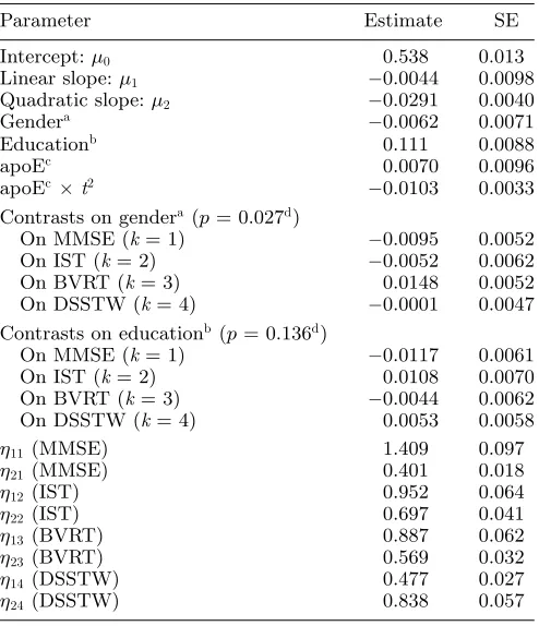
[image:5.612.302.546.110.194.2]Using the beta transformation, the best fitting model included a quadratic function of time with three random coefficients and the three covariates (educational level, gender, and apoE
Table 1
Fit of the data for various transformations in the model without covariates and a quadratic function of time
Number of Log
Family of transformation parameters likelihood AIC
Linear transformation 20 −21584.1 43208.2
Beta CDF 22 −20387.1 40818.2
Logit + 20 −20876.4 41792.8
linear transformation
Weibull CDF 22 −20654.7 41353.4
[image:5.612.301.548.406.693.2]genotype) in the model for the latent process. As it was sus-pected that ability in visual memory, verbal fluency, and at-tention could be differently associated with gender and educa-tional level, we also included contrasts between tests for these covariates. Interactions between apoE genotype and time vari-ables were also included in the latent process. Interactions between gender and time and between educational level and time were not found to be significant and did not confound the association between apoE and cognitive evolution. Thus they were excluded from the final model. Estimates of the fixed effect parameters in the final model are presented in Table 2.
Table 2
Estimates of the fixed effect parameters in the best model with
the beta transformation(log likelihood=−19715.55;number
of parameters= 36;AIC= 39503.1)
Parameter Estimate SE
Intercept:μ0 0.538 0.013
Linear slope:μ1 −0.0044 0.0098
Quadratic slope:μ2 −0.0291 0.0040
Gendera −0.0062 0.0071
Educationb 0.111 0.0088
apoEc 0.0070 0.0096
apoEc×t2 −0.0103 0.0033
Contrasts on gendera (p= 0.027d)
On MMSE (k= 1) −0.0095 0.0052
On IST (k= 2) −0.0052 0.0062
On BVRT (k= 3) 0.0148 0.0052
On DSSTW (k= 4) −0.0001 0.0047
Contrasts on educationb(p= 0.136d)
On MMSE (k= 1) −0.0117 0.0061
On IST (k= 2) 0.0108 0.0070
On BVRT (k= 3) −0.0044 0.0062
On DSSTW (k= 4) 0.0053 0.0058
η11(MMSE) 1.409 0.097
η21(MMSE) 0.401 0.018
η12(IST) 0.952 0.064
η22(IST) 0.697 0.041
η13(BVRT) 0.887 0.062
η23(BVRT) 0.569 0.032
η14(DSSTW) 0.477 0.027
η24(DSSTW) 0.838 0.057
aReference: female.
bReference: not graduated from primary school.
cReference:4 noncarrier.
dLikelihood ratio test for the contrast variables (X2with 3 degrees
The test-specific random effectsαik dramatically improved the fit (574 increase of the log likelihood for four additional parameters), which means that for a same value of latent cognition, subjects score differently in cognitive domains asso-ciated with the psychometric tests. Accounting for the within-subject variability with a Brownian motion was also relevant since it increased the log likelihood of 13.8.
Gender was not significantly associated with the mean com-mon factor level, while subjects who graduated from primary school had a significantly better mean common factor level. Inclusion of contrasts between tests for gender improved sig-nificantly the fit of the model, showing that gender does not have the same impact on each psychometric test: men tend to perform better on the BVRT than women, while the trend is reversed for the other tests. Contrasts between tests for educational level are not significant, which suggests that the effect of educational level does not differ from test to test.
The apoE genotype was only included in the latent process evolution (equation (1)) because the hypothesis to evaluate was an association between the 4 allele and the decline of latent cognitive performance. We had no hypothesis
0 0.2 0.4 0.6 0.8 1
0 5 10 15 20 25 30
g(MMSE)
MMSE
0 0.2 0.4 0.6 0.8 1
0 5 10 15 20 25 30 35 40
g(IST)
IST
0 0.2 0.4 0.6 0.8 1
0 2 4 6 8 10 12 14
g(BVRT)
BVRT
0 0.2 0.4 0.6 0.8 1
0 10 20 30 40 50 60 70
g(DSSTW)
[image:6.612.70.570.341.700.2]DSSTW
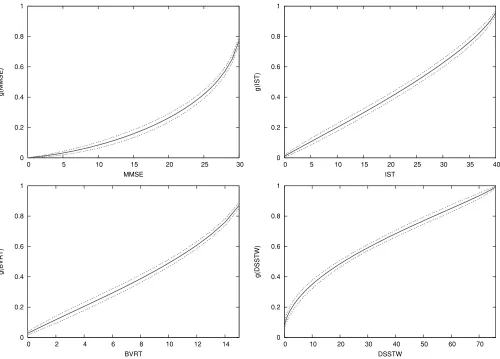
Figure 2. Estimated beta transformation for each test (solid line) and the 95% pointwise confidence interval (dashed line, obtained by bootstrap).
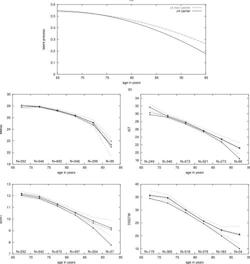
ing a link with a specific psychometric measure. We found no association between the4 allele and the mean level of the common factor at age 65 years but found a strong association (p= 0.0018) with the change over time of the common fac-tor:4 carriers have a steeper decline than4 noncarriers as shown in Figure 4a. The model including both the interactions apoE× tand apoE× t2 had exactly the same likelihood as
the model including only apoE × t2. Thus we retained the
latter.
Figure 2 displays the estimated beta transformations for the four tests with the 95% pointwise confidence interval com-puted using a bootstrap method. The four estimated transfor-mations are very different: the curve is convex for the MMSE and the BVRT, concave for the DSSTW, and close to lin-ear for the IST. Moreover, the BVRT and the MMSE scores cover, respectively, only 80% and 88% of the latent process range while the DSSTW covers around 95% and the IST cov-ers almost the entire range.
process lower than its maximum. These estimated curves highlight the ceiling effect of the two tests. More generally, the nonlinear shape of the MMSE reveals that a decline in the MMSE should be interpreted by taking the initial level into account: one point lost from a score above 25 represents a more substantial decrease of cognition (about 0.06) than one point lost from a score under 15 (about 0.01). For the DSSTW, the curve is close to linearity above a score of 10 but one point lost under a score of 10 represents a more sub-stantial decrease of the latent cognition. Subjects with a latent cognition lower than 0.1 tend to score 0 on the DSSTW, prob-ably because they do not even understand the instructions. In contrast, the IST appears to be useful to evaluate cognition in a heterogeneous population including high-level and impaired subjects, because it is close to linearity on almost the entire range of the latent cognition.
[image:7.612.47.550.340.702.2]5.4 Assessment of the Fit
Figure 3 contains the normal quantile plots of the standard-ized marginal residuals defined in (9) for each of the four psy-chometric tests. The normality assumption of the residuals seems to be well satisfied for each of the four psychometric
-6 -4 -2 0 2 4 6
-4 -3 -2 -1 0 1 2 3 4
MMSE
-6 -4 -2 0 2 4 6
-4 -3 -2 -1 0 1 2 3 4
IST
-6 -4 -2 0 2 4 6
-4 -3 -2 -1 0 1 2 3 4
BVRT
-6 -4 -2 0 2 4 6
-4 -3 -2 -1 0 1 2 3 4
DSSTW
Figure 3. Normal quantile plot of the standardized marginal residuals for each test (solid lines = “y = x” reference line and 95% confidence interval).
tests. In contrast, when using a linear transformation, nor-mal quantile plots showed a poor agreement with the nornor-mal assumption (results not displayed).
0 0.1 0.2 0.3 0.4 0.5 0.6
65 70 75 80 85 90 95
latent process
age in years (a)
ε4 non carrier ε4 carrier
18 20 22 24 26 28 30
65 70 75 80 85 90 95
MMSE
age in years
(b)
N=252 N=546 N=692 N=546 N=299 N=99 18
20 22 24 26 28 30 32 34
65 70 75 80 85 90 95
IST
age in years
N=249 N=540 N=673 N=521 N=273 N=80
7 8 9 10 11 12 13
65 70 75 80 85 90 95
BVRT
age in years
N=252 N=542 N=670 N=497 N=254 N=57 15
20 25 30 35 40
65 70 75 80 85 90 95
DSSTW
age in years
[image:8.612.68.568.81.609.2]N=179 N=360 N=518 N=379 N=183 N=34
Figure 4. (a) Predicted mean evolution for the latent process for4 carriers and for 4 noncarriers. (b) Estimated and observed mean evolutions for each test with the number of subjects used for the computation of each observed mean (solid line with crosses = observed mean evolution; solid line with dots = estimated marginal mean evolution; dashed line with dots = estimated subject-specific mean evolution; dashed line = 95% confidence interval of the observed mean).
cognitive level tended to refuse the other tests and particu-larly the DSSTW, which is more difficult. Missing data are thus associated with random effects. For instance, the mean of subject-specific deviations ˆWijkis−0.0037 for subjects aged
has previously been discussed by Molenberghs and Verbeke (2001).
5.5 Multivariate Model versus Univariate Models
For each test, the univariate model detected an association between apoE genotype and cognition with a larger p-value (p-value from the likelihood ratio test for apoE×t2
param-eter: p = 0.0043 for MMSE, p = 0.018 for IST, p = 0.020 for BVRT, p = 0.054 for the DSSTW) than for the multi-variate model (p = 0.0018). By using a multivariate model compared to four univariate models, we had a gain of power in assessing the association between apoE genotype and cog-nition. Moreover, note that interpretation of the association with the latent process and with each psychometric test is different.
The gain in efficiency can also be evaluated by comparing the AIC from the multivariate model and the AIC computed by pooling the likelihoods from the four univariate models with the total number of parameters in these four models. In our case, even if we added in the multivariate model the constraint that apoE had a common effect on the four tests, the AIC from the multivariate model was markedly better (39503.1 vs. 40203.8 for the four univariate models).
6. Discussion
We proposed a nonlinear model for multivariate longitudinal non-Gaussian quantitative outcomes when the outcomes are indirect measures of a common underlying continuous-time process. Such data are very frequent in psychometrics, but the methodology has many other potential areas of application, as, for instance, the study of the course of chronic illnesses evaluated by several biological markers.
In this work, psychometric tests are analyzed by consid-ering their sum scores as quantitative variables. This is the most frequent way to consider psychometric tests in geron-tology: the summary scores are used to evaluate cognitive level and risk of dementia (Hall et al., 2001; Sliwinski et al., 2003; Amieva et al., 2005). From a neuropsychological perspective, the alternative approach, which consists of an-alyzing item responses using SEM or item response model (Skrondal and Rabe-Hesketh, 2004, Chapter 3), could be use-ful if the objective was to understand the underlying compo-nents of the tests. This methodology is interesting when the tests consist of a limited number of items evaluating different cognitive domains (such as the MMSE) or exhibiting differ-ent levels of difficulty (such as the BVRT). On the contrary, this methodology would be difficult to apply to the IST score, which is the number of words cited by the subjects (except for considering the four subscores for each semantic category) and the DSSTW score, which is the count of symbols correctly assigned to a sequence of numbers.
Given that the summary scores are quantitative discrete variables, we could either consider them as continuous vari-ables or as ordinal varivari-ables. However, threshold models for ordinal data require estimation of one threshold for each pos-sible value of the scores, which would be very challenging for multivariate modeling of scores with so many different val-ues. In our application including four tests, this would have implied estimation of more than 150 additional parameters. Thus, we decided to analyze the scores as continuous variables
and to use nonlinear transformations depending on a limited number of parameters as link functions between the Gaus-sian latent process and the observed outcomes. Various link functions have been considered, but we found that the beta CDF was flexible enough with only two parameters. With many fewer parameters than threshold models, the estimated curves provide interesting information on the relationship be-tween evolution of the latent cognitive level and evolution of the observed scores. Moreover, goodness-of-fit analyses show that the beta transforms of the four test scores fitted well a Gaussian distribution. Nevertheless, if necessary for other applications, it would be easy to include a different family of continuous transformation for each test. This model could also be extended to allow a mixture of continuous, binary, and ordinal outcomes with few categories as in Dunson (2000), Dunson (2003), or Rabe-Hesketh et al. (2004).
Another asset of this model is the way of accounting for covariate effects. Using fixed contrasts, we were able to distin-guish between the association with the latent process and the differential association with the various psychometric tests. Being able to compare covariate effects over the tests is also an advantage of multivariate modeling. With a large number of tests it may also be possible and advantageous to have the effects of the covariates on the tests be random rather than fixed.
We assumed the data to be missing at random and thus ignorable using a maximum likelihood approach. Even if we have shown that missing data were associated with random effects, this does not preclude missing data from being ignor-able. Indeed, if missing data at the last three tests depend on the observed MMSE score or on the observed evolution of the MMSE, it induces a dependency on the random effects, but the missing data are ignorable because missing values may be predicted using observed data. This is an advantage of multivariate modeling, in that by using more observed infor-mation it is more robust to missing data. Nevertheless, as it is not excluded that missing data are informative, it could be useful to jointly model time to dropout using a shared ran-dom effect model as in Roy and Lin (2002). However, this would increase complexity of the estimation process and esti-mates would depend on uncheckable parametric assumptions. Another useful extension would be to jointly model demen-tia, defining dementia diagnosis as the time at which the la-tent process first reaches an estimated threshold (Hashemi, Jacqmin-Gadda, and Commenges, 2003).
Acknowledgements
The authors thank Jean-Fran¸cois Dartigues, Luc Letenneur, and the PAQUID research team for providing the data.
References
Amieva, H., Jacqmin-Gadda, H., Orgogozo, J., LeCarret, N., Helmer, C., Letenneur, L., Barberger-Gateau, P., Fabrigoule, C., and Dartigues, J. (2005). The 9 year cog-nitive decline before dementia of the Alzheimer type: A prospective population-based study. Brain 128, 1093– 1101.
and the Metropolis-Hastings algorithm. Psychometrika 63,271–300.
Dunson, D. (2000). Bayesian latent variable models for clus-tered mixed outcomes. Journal of the Royal Statistical
Society, Series B62,355–366.
Dunson, D. (2003). Dynamic latent trait models for multi-dimensional longitudinal data. Journal of the American
Statistical Association98,555–563.
Fabrigoule, C., Rouch, I., Taberly, A., Letenneur, L., Commenges, D., Mazaux, J.-M., Orgogozo, J.-M., and Dartigues, J.-F. (1998). Cognitive process in preclinical phase of dementia.Brain121,135–141.
Farrer, L., Cupples, L., Haines, J., Hyman, B., Kukull, W., Mayeux, R., Myers, R., Pericak-Vance, M., Risch, N., and Van Duijn, C. (1997). Effects of age, sex and eth-nicity on the association between apolipoprotein E geno-type and Alzheimer disease. A meta-analysis. APOE and Alzheimer Disease Meta Analysis Consortium.Journal of
the American Medical Association278,1349–1356.
Gray, S. M. and Brookmeyer, R. (1998). Estimating a treat-ment effect from multidimensional longitudinal data.
Biometrics54,976–988.
Hall, C., Ying, J., Kuo, L., Sliwinski, M., Buschke, H., Katz, M., and Lipton, R. (2001). Estimation of bivariate mea-surements having different change points, with applica-tion to cognitive ageing.Statistics in Medicine20,3695– 3714.
Harvey, D., Beckett, L., and Mungas, D. (2003). Multivariate modeling of two associated cognitive outcomes in a lon-gitudinal study.Journal of Alzheimer’s Disease 5,357– 365.
Hashemi, R., Jacqmin-Gadda, H., and Commenges, D. (2003). A latent process model for joint modeling of events and marker.Lifetime Data Analysis9,331–343.
Jacqmin-Gadda, H., Fabrigoule, C., Commenges, D., and Dartigues, J.-F. (1997). A 5-year longitudinal study of the Mini Mental State Examination in normal aging.
American Journal of Epidemiology145,498–506.
J¨oreskog, K. and Yang, F. (1996). Nonlinear structural equa-tion models: The Kenny-Judd model with interacequa-tion ef-fects. In Advanced Structural Equation Modeling: Issues
and Techniques, G. A. Marcoulides and R. E. Schumacker
(eds), 57–88. Mahwah, New Jersey: Lawrence Erlbaum Associates.
Kendall, M. and Stuart, A. (1977).The Advanced Theory of
Statistics, Volume 1. New York: MacMillan Publishing.
Lee, S. and Song, X. (2004). Bayesian model comparison of nonlinear structural equation models with missing con-tinuous and ordinal categorical data. British Journal of
Mathematical and Statistical Psychology57,131–150.
Letenneur, L., Commenges, D., Dartigues, J.-F., and Barberger-Gateau, P. (1994). Incidence of dementia and Alzheimer’s disease in the elderly community residents of south-western France.International Journal of
Epidemi-ology23,577–590.
Longford, N. and Muth´en, B. (1992). Factor analysis for clus-tered observations.Psychometrika57,581–597.
Marquardt, D. (1963). An algorithm for least-squares estima-tion of nonlinear parameters. SIAM Journal on Applied
Mathematics11,431–441.
Molenberghs, G. and Verbeke, G. (2001). A review on linear mixed models for longitudinal data, possibly subject to dropout.Statistical Modelling1,235–269.
Muth´en, B. (2002). Beyond SEM: General latent variable modeling.Behaviormetrika29,81–117.
Rabe-Hesketh, S., Skrondal, A., and Pickles, A. (2004). Gen-eralized multilevel structural equation modelling.
Psy-chometrika69,167–190.
Roy, J. and Lin, X. (2000). Latent variable models for lon-gitudinal data with multiple continuous outcomes.
Bio-metrics56,1047–1054.
Roy, J. and Lin, X. (2002). Analysis of multivariate longitu-dinal outcomes with nonignorable dropouts and missing covariates: Changes in methadone treatment practices.
Journal of the American Statistical Association 97, 40–
52.
Salthouse, T., Hancock, H., Meinz, E., and Hambrick, D. (1996). Interrelations of age, visual acuity, and cogni-tive functioning. Journal of Gerontology: Psychological
Sciences51B,317–330.
Sammel, M. and Ryan, L. (1996). Latent variable models with fixed effects.Biometrics52,650–663.
S´anchez, B. N., Budtz-Jorgensen, E., Ryan, L. M., and Hu, H. (2005). Structural equation models: A review with applications to environmental epidemiology. Journal of
the American Statistical Association100,1443–1455.
Skrondal, A. and Rabe-Hesketh, S. (2004).Generalized Latent Variable Modelling: Multilevel, Longitudinal and
Struc-tural Equation Models. Boca Raton, Florida: Chapman
& Hall/CRC.
Sliwinski, M., Hofer, S., and Hall, C. (2003). Correlated and coupled cognitive change in older adults with or without preclinical dementia.Psychology and Aging18,672–683. Song, X. and Lee, S. (2004). Bayesian analysis of two-level nonlinear structural equation models with continuous and polytomous data. British Journal of Mathematical
and Statistical Psychology57,29–52.
Wall, M. and Amemiya, Y. (2000). Estimation for polynomial structural equation models.Journal of the American
Sta-tistical Association95,929–940.
Winnock, M., Letenneur, L., Jacqmin-Gadda, H., Dallongeville, J., Amouyel, P., and Dartigues, J. (2002). Longitudinal analysis of the effect of apolipopro-tein E 4 and education on cognitive performance in elderly subjects: The PAQUID study. Journal of
Neurology, Neurosurgery and Psychiatry72,794–797.
Yalcin, I. and Amemiya, Y. (2001). Nonlinear factor analysis as a statistical method.Statistical Science16,275–294.
Received January2005.Revised December2005.
Accepted January2006.
Appendix
Details on the Transformations
For subjectiand testk, we give the expressions of the function and its Jacobian for the linear transformation, the combina-tion of a linear and a logit transformacombina-tion, and the Weibull CDF.
gk(y;η1k, η2k) =
y−η1k η2k
J(yi;θ) = K
k=1
1 η2k
.
The combination of a linear and a logit transformation is de-fined fory∈(0, 1),η1k ∈(0, 1), andη2k ∈(0, 1) as
gk(y;η1k, η2k) =
ln
y 1−y
−ln
η1k 1−η1k
ln
η2k 1−η2k
J(yi;θ) = K
k=1
nik
j=1
1
ln
η2k 1−η2k
yijk(1−yijk) .
The Weibull CDF is defined fory∈(0,∞),η1k∈(0,∞), and η2k ∈(0,∞) as
g(y;η1k, η2k) = 1−exp
−
y η1k
η2k
J(yi;θ) = K
k=1
nik
j=1
η2kyη2k−1 ηη2k
1k
exp
−
y η1k
η2k