2018 International Conference on Computational, Modeling, Simulation and Mathematical Statistics (CMSMS 2018) ISBN: 978-1-60595-562-9
Image Change Detection and Statistical Test
Wen-Yu WANG
1, Wei-Hua FANG
2,*, Guo-Yin CAI
1, Ping-jun NIE
1and Dong-xin LIU
11Beijing University of Civil Engineering and Architecture, Beijing, China
2Key Laboratory of Environmental Change and Natural Disaster, Ministry of Education,
Beijing Normal University, Beijing, China *Corresponding author
Keywords: Land change, Binary image change detection, Hypothesis test, Phenology problem.
Abstract. Image change detection, a technique in distinguishing “change/no change” area, can be regarded as a process of decision which can be solved by constructing hypothesis tests. Co-registered paired images (before image and after image) were studied in this report by exploring the standard steps of hypothesis test. Differencing of biomass index (dNDVI) is selected to denote the change variable considering its advantage of maximizing the spectral difference between vegetation and man-made features. Since this was a before-and-after study, t-test for paired observations was established. Adopting statistical test as inferential tool, land change decisions were made to incorporate both land change signals and noises. However, under complex spatial circumstance, many assumptions can be violated. After achieving the change decisions, spatial correlation and phenology problem were further checked as extreme outlier might lead to a false decision. Results indicate that phenology problems can pollute the change decisions and need to be further isolated in future studies.
Introduction
Image Change Detection (CD) techniques, identifying differences in temporal images, are useful in many computer-based applications, such as video surveillance, medical imaging and remote sensing, where quick responses are highly demanded [2, 6, 10]. In remote sensing applications, Land Use and Cover Change (LUCC) studies, aiming at a better understanding of the relationships and interactions between human and natural phenomena, are heavily depending on image techniques, especially for large extensive area in recent decades [6, 7]. In this study, land cover change (2010 to 2015) in Beijing metropolitan area was tentatively explored using bi-temporal Landsat images.
To choose an appropriate method to construct change image is the most important thing in change detection. Among various image CD algorithms, two categories can be identified: “spectral-based algorithms” and “post-classification algorithms”. The main difference between these two categories is to detect first or to classify first. “Spectral-based algorithms” detect first without classification information, while “post-classification algorithms” classify first and thematic information will be used in change detection. In this study, pre-classification change detection was used due to the effectiveness and efficiency of image algebra and image transformation. Among spectral-based algorithms, some simple algorithms, such as image differencing techniques, can achieve higher accuracy than sophisticated methods, such as principal component analysis (PCA) [12, 14]. In this study, the univariate image differencing techniques will be used to construct change image.
Data and Methods
A sub-area of Beijing during the time span (2010-2015) was chosen for this pilot study. Several parameters were considered during choosing Landsat images: (1) sensor selection, (2) date selection, (3) cloud cover < 20%, (4) quality = 9. One pair of images (Landsat 5 TM 2010_06_05 and Landsat 8 OLI 2015_04_16) was selected. To produce binary change image, this pair of images will undergo four procedures: preprocessing, image analysis, statistical test and post-processing.
Pre-processing
In the preprocessing stage, the atmospheric correction is applied to remove scattering and absorption effects before quantitative analysis of multi-date and multi-sensory images. Two steps were taken to change the two raw images to “clear” images. Firstly, the DNs of the two Landsat scenes were rescaled to the top of atmosphere (TOA) reflectance. Secondly, the surface (ground) reflectance free from atmospheric effect was computed using “black object subtraction” tool in ENVI 5.2[4].
Image Analysis
The Normalized Difference Vegetation Index (NDVI), a standardized index of greenness (relative biomass), was chosen as the change variable for bi-temporal images. In ArcGIS Image Analysis, if “Scientific output” is checked, the NDVI output values are between -1.0 and 1.0. Otherwise the NDVI function will scale the values to a range of 0–200 (Eq. 1), which can easily be rendered with a specific color ramp or color map.
NDVI = ((NIR - red)/ (NIR + red)) * 100 + 100 (1) By subtracting two NDVI images, the differencing NDVI (dNDVI) can be achieved. And the normality of it can be checked by histogram.
Hypothesis test
As change was expected to be found in paired images, the null hypothesis is established as there are no changes between two images. By rejecting the null hypothesis, we reach the change decision. Z-statistic was chosen based on the assumption of the normal distribution of the change variable, dNDVI. Paired t-test statistic is calculated as follows:
𝑡= (2) Where d𝑁𝐷𝑉𝐼 = the difference of NDVI between two images,e = the expected value of dNDVI,
s = the standard deviation of dNDVI.
Post-processing
In the final stage of post-processing, the change area was masked out to further study the phenology problem. The original spectral histogram was graphed to investigate more problems concerning the phenology. By checking the original NDVI in two scenes, it is easy to distinguish those change areas that are subjective to vegetation and those change area that are not due to the phenology change.
Results and Discussion
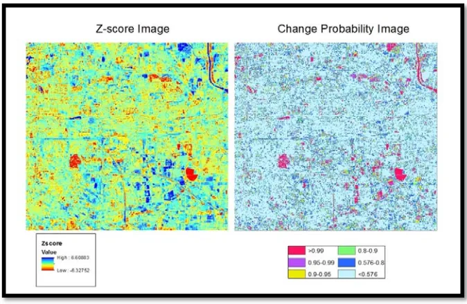
Figure 1. Z-score Image and Change Probability Image.
Theoretically, any Z-score value has an according p-value and can be achieved through some numerical analyses. However, in most cases, only approximate values can be got on a table of standard values (z table). So technically, the exact p-value for a given z-score cannot be got. To solve such inconvenience, two steps were adopted: (1) Designate probability values (0.99, 0.95, 0.90, 0.80, 0.576) and find the according critical z-values from a z-table. To facilitate the re-classification in ArcGIS, the float z-scores were converted to integer value by multiplying 100. (2) Interval levels were set on z-scores and the according probability values (Table 1). Through the above two steps, the relationship between z-score interval level and probability interval level was established.
[image:3.612.93.522.527.642.2]Figure 1 (right) below shows the change probability distribution. Instead of “hard” thresholding, hypothesis test produce “soft” decisions using probabilities. A probability can be regarded as the frequencies of success happening in the long run [5]. Comparing to binary decisions, this map can possess more information on change decision process, because probabilities not only illustrate the strength of change decision, but also denote the uncertainty in our decisions. Errors and uncertainties are the nature of change process. However, hard thresholding technique totally loses such useful information.
Table 1. Probability zoning strategies.
Zoning Z-scores Probability (Confidence level) Confidence Grade
-80<Z-score*100 <80 <0.576 6
-128<Z-score*100<-80 or 80<Z-score*100<128 0.576-0.8 5
-165<Z-score*100<-128 or 128<Z-score*100<165 0.8-0.9 4
-196<Z-score*100<-165 or 165<Z-score*100<196 0.9-0.95 3
-258<Z-score*100<-196 or 196<Z-score*100<258 0.95-0.99 2
Z-score*100<-258 or Z-score*100>258 >0.99 1
signal of real land cover change. Without breaking these two types of signals apart, it is hard to present a satisfactory work.
Figure 2. Biomass decrease and increase pixels overlaid on 2015 NDVI image.
Detection of image differences may be confused with problems in penology and cropping, and such problems may be exacerbated by limited image availability, poor quality in temperate zones and difficulties in calibrating poor images [1]. Among many methods that can deal with the phenology problem, the idea of cross correlation method is widely used by adopting an existing Date 1 land-cover map and a Date 2 multispectral image and it can well solve the radiometric and phenology differences as only one image was used in the study[2,9,13]. To produce the NLCD 2011, Jin et al. (2013) designed zone model to capture subtle change in forest area that change is mainly due to phenology and seasonal change.
Conclusions
In this study, image ratio differencing and statistical test were adopted to make decisions on change area on the bi-temporal Landsat images. From the positive sides, NDVI differencing is straightforward and practical: (1) NDVI has the advantage of maximizing the spectral difference between vegetation and man-made features; (2) Univariate image analysis does not need to concern about the redundancy among multispectral bands; (3) The distribution of dNDVI is roughly bell-shape, indicating that changes randomly took place across the research area and dNDVI should be a random variable, the value of which is a combination of true signal and random noise. This is the basis of hypothesis test, although it can be easily violated by spatial variable due to the spatial autocorrelation and spatial heterogeneity. Furthermore, hypothesis test, as inferential statistic, can handle noises and uncertainties in image change detection. The advantages of hypothesis test can be summarized as follows: (1) Instead of hard binary change decision, the hypothesis test can produce a soft probability change decision; (2) Change probability can simultaneously denotes the strength of decision and uncertainty; (3) From a frequentist perspective, probability is regarded as the long-run frequency of an outcome occurring, while from a Bayesian perspective, probability quantifies a degree of belief in our decisions. Such idea strengthens our determination to establish land use class frequencies as prior probabilities, instead of worrying about the assumption of fixed mean from samples or population.
failed to calibrate two images to the same conditions: (1) Paired images have different air conditions, however the available atmospheric correction algorithm cannot remove the haze and fog in the low height; (2) Paired images are from different sensors, it is necessary to calibrate two NDVI images. Another problem is phenology problem. The phenology change is regarded as the pseudo change or spurious change, not the real land cover change. However the signal of phenology change of vegetation intertwined with the real land change information. Without breaking these two signals apart, it is hard to present a satisfactory result. Or in other words, the assumption that “difference is the composite of errors and changes” is not practicable in land cover change detection.
Last but not least, although hypothesis test is a useful inferential tool that can handle errors and uncertainties in modeling, but it usually depends on the known distribution of the change variable. In many cases, the distribution of the change variable may not be known, or it does not perfectly follow the expected distribution. Another inferential tool-sensitivity analysis will be studied in the future.
Acknowledgement
This work is supported by the National Key Research and Development Program of China under Grant 2017YFA0604903.
References
[1] Boori, M.S., & Amaro, V.E. (2010). Land use change detection for environmental management: using multi-temporal, satellite data in Apodi Valley of northeastern Brazil. Applied GIS, 6(2), 1-15. [2] Canty, M.J. (2014). Image analysis, classification and change detection in remote sensing: with algorithms for ENVI/IDL and Python. CRC Press.
[3] Civco, D.L., Hurd, J.D., Wilson, E.H., Song, M., & Zhang, Z. (2002, April). A comparison of land use and land cover change detection methods. In ASPRS-ACSM Annual Conference.
[4] ENVI 5.2 (2016), Retrieved from envi5.2 tutorial.
[5] Harris, R., & Jarvis, C. (2014). Statistics for geography and environmental science. Routledge. [6] İlsever, M., &Unsalan, C. (2012). Two-Dimensional Change Detection Methods: Remote Sensing Applications. Springer Science & Business Media.
[7] Jensen, J. R. (2015). Introductory digital image processing: a remote sensing perspective. Pearson College Division.
[8] Jin, S., Yang, L., Danielson, P., Homer, C., Fry, J., & Xian, G. (2013). A comprehensive change detection method for updating the national land cover database to circa 2011. Remote Sensing of Environment, 132, 159-175.
[9] Koeln, G., & Bissonnette, J. (2000, May). Cross-correlation analysis: mapping landcover change with a historic landcover database and a recent, single-date multispectral image. In Proc. 2000 ASPRS Annual Convention, Washington, DC.
[10] Nika, V., Babyn, P., & Zhu, H. (2014). Change detection of medical images using dictionary learning techniques and principal component analysis. Journal of Medical Imaging, 1(2), 024502-024502.
[11] Siewe, S.S. (2007). Change Detection Analysis of the Landuse and Landcover of the Fort Cobb Reservoir Watershed. ProQuest.
[13] Tarantino, C., Adamo, M., Lucas, R., & Blonda, P. (2016). Detection of changes in semi-natural grasslands by cross correlation analysis with WorldView-2 images and new Landsat 8 data. Remote Sensing of Environment, 175, 65-72.