2018 International Conference on Computer, Communication and Network Technology (CCNT 2018) ISBN: 978-1-60595-561-2
A Multi-Objective Chaotic Particle Swarm Optimization Algorithm
Based on Improved Inertial Weights
Zhi-yuan PAN, Da-min ZHANG
*, Dong LIU, Jun YANG and Juan-min CHEN
College of Data and Information engineering, Guizhou University, Guiyang, Guizhou, 550025, PR China
*Corresponding author
Keywords: Multi-Objective particle swarm optimization algorithm, Logistic map, Elite archiving mechanism, Mutation probability.
Abstract. In order to enhance the convergence and distribution of multi-objective particle swarm algorithm, an improved multi-objective particle swarm optimization algorithm was proposed. Linear decreasing inertia weight was used to update. The method can improve the deficiency that the algorithm falls into local optimal easily. The improved Logistic mapping was used to increase ergodicity of the particles. The method can expand the search scope. At the same time, the elite archiving mechanism and the mutation probability were introduced to increase the disturbance. The method can improve the local optimal. Compared with the real Pareto front, NSGA-II and MOEAD algorithm, the simulation shows that the algorithm proposed in the paper is effective.
Introduction
There are many optimization problems in real life, and meanwhile, the optimization problems need to optimize multiple objectives at the same time. In general, the multiple objective functions in the same problem are contradictory and interaction[1]. So the final results are a series of compromise solutions being called Pareto optimal solutions sets or non-dominated solution sets.
Because particle swarm optimization (PSO) has the features of less parameter, good optimization performance, and fast convergence speed. It has been widely concerned and been successfully applied in many fields such as function optimization, data mining and wireless sensor network in recent years.
Focusing on the research status at home and abroad, the main research results are summarized as improving the updating strategy of external archive, the selection strategy of global guide, combining the particle swarm algorithm with other algorithms and so on. In literature [2], the external particles were used to guide the flight of the population particles, and the optimal solutions in the group search process were stored in a file. The algorithm is easy to fall into the local optimum being used to optimize multi-peak function. In literature [3], ε-domination was introduced to
determine the global extremum of particles. The method can improve the diversity and the uniformity of particles distribution. In literature [4], the preference ε-Pareto domination was introduced to short search time and enhance convergence. In literature [5], a dynamic domain strategies and new particle memory strategies were adopted in the algorithm. In literature [6], a multi-objective interactive PSO algorithm was proposed. To maximize the non-dominated solutions with the adaptive grid mechanism, adaptive mutation operation and user decision functions were used in the algorithm. In literature [7], Pareto entropy was proposed to assess population diversity and current evolutionary states. The evolution strategy can be designed to balance the convergence and diversity with the Pareto entropy. In literature [8], a multi-sub-population co-evolution mechanism was proposed. An external archive and elite learning strategies were introduced to improve distribution and convergence of the algorithm. In literature [9], Chaotic sequence was used to initialize population. The population can be more evenly distributed in the decision space with the method.
the optimal location, Elite archiving strategy was used to archive non-dominated solutions, the crowd distance between particles was calculated and in descending order, the mutation probability was introduced to perturb the particles to increase convergence and diversity of the algorithm.
The paper is organized as follows: The theoretical basis is described in Section 2. The improved algorithm is presented in Section 3. Simulation results and analysis are provided in Section 4. Conclusions are drawn in Section 5.
Theoretical Basis
Multi-Objective Optimization
Generally, a multi-objective optimization problem with d decision variables and k target variables
can be expressed as follows[10]:
1 2
min ( ) ( ( ), ( ),..., ( ))
. . ( ) 0, 1, 2,...,
h ( ) 0, 1, 2,...,
T k
i
j
y F x f x f x f x
s t g x i q
x j p
= =
≤ =
= =
(1)
Where ( ,..., )1
n n
x=x x ∈ ⊂X R is d-dimensional decision vector, X is d-dimensional decision space.
1
( ,..., ) k
m
y= y y ∈ ⊂Y R is k-dimensional target vector, Y is k-dimensional target space. Objective
function F x( ) is defined as mapping from the k decision space to the target space.
Basic Particle Swarm Optimization Algorithm
The basic particle swarm optimization algorithm (PSO) is an optimization algorithm based on swarm intelligence theory, which was proposed by Kennedy and Eberhart in 1995[9]. The PSO simulates the bird’s behavior of randomly searching for food[11]. In PSO algorithm, every particle represents a potential solution and it has a fitness value determined by objective functions. Meanwhile every particle has a velocity to determine the direction and distance of “flying”. The particles can follow current optimal particle to find the optimal solution by iteration. The update formula is as follows:
1 1( ) 2 2( )
id id id id gd id
v = ∗ω v +c r p −x +c r p −x
(2)
id id id
x =x +v
(3) Where vid and xid represent current velocity and position of the i particle. pid is personal best
particle. pgd is global best particle. ω is inertia weight of particle. c1 and c2are learning factors.
1
r and
2
r are random numbers distributed in [0,1].
Generally, at the beginning of iteration, the larger inertia weight is more beneficial for global search, and at the later stages of iteration, smaller inertia weights can enhance local searching ability. A method of linear decreasing inertia weight is used in this paper, and defined as follows:
min max min
= ( )MaxIt it
MaxIt
ω ω + ω −ω −
(4) In the above formula, it is current the population iteration. MaxIt is the total number of
population iterations. ωmin is the minimum inertia weight. ωmax is the maximum inertia weight.
A Multi-Objective Chaotic Particle Swarm Optimization Algorithm Based on Improved Inertial Weights
Chaos Optimization
method can prevent the algorithm from falling into local optimum[12]. An improved chaotic Logistics mapping function is used in this paper, and it is defined as:
2 1 1 2
n n
x x
+ = − × (5)
Where x0 is in the range of [0,1]. In this paper, the optimal solutions in the archive are mapped
into the definition domain of formula (5). The chaotic sequences are generated by iteration according to the mapping formula, and then are returned to the original solution space by inverse mapping. The fitness value of the new solutions can be calculated and the best solutions are released into the archive.
Elite Archiving Mechanism
In traditional single-objective evolutionary algorithms, the individual with large fitness tends to be elite individual which are directly copied to the next generation without crossover and mutation and so on[13]. According to the elite archival strategy, the superiority or inferiority particle is determined based on the corresponding dominated degree of target vector of particle. If the new particle dominates the particle in the archive, the dominated particle can be replaced by the new particle. If the new particle is dominated by particle in the archive, the new particle can't be put into the archive. If the new particle and the particle in the archive are not dominated each other, the new particle can be put into the archive.
Mutation Strategy
In the early stages of search, it is not easy to obtain a local optimum. Oppositely, as the iteration progress, it is very difficult for particle to jump out of the local optimum based on its knowledge and social behavior. Above this, a mutation strategy is introduced. The particle position can be disturbed in a small range according to a certain probability. The particle mutation probability being called Pm is determined according to the number of iteration. The mutation probability and
disturbance formulas are as follows:
2
(1 ( 1) / ( 1))
m
P = − it− MaxIt−
(6)
max min
( )
d d d d
i i
x =x ∗ x −x +σ
(7) Where max
d
x and
min
d
x are the upper and lower bounds of the particle in the d-dimension. σ is
the uniformly distributed random number between [0,1]. In formula (6), the mutation probability of particles increases with the number of iteration increases. At the later iteration, the probability is gradually reduced, which can effectively avoid the error judgment for local optimum and mutation.
Crowding Distance
Crowding distance is used to estimate the density of other solutions around a solution. For every objective function, the non-inferior solutions of the elite solution set are sorted in descending order according to the fitness value. Let the distance between the first and last particles is infinite, then calculate the crowding distance. Being inspired by Euclidean distance, an improved crowding distance is defined as follows:
2
max min 1
( 1) ( 1)
row ( )
d
m m
i
m m m
f i f i
f f
=
− − +
=
−
∑
(8) Where, fm(i−1) and fm(i+1)represent the fitness value of two adjacent particles in m-dimensions
respectively. max
m
f and min
m
f represent the maximum and minimum fitness values of particle in
The Algorithm Flow
The steps of the multi-objective particle swarm algorithm process are as follows:
Step 1: Initialize the population size N and the number of iteration, set the parameters of the
algorithm and the number of chaotic optimization.
Step 2: Randomly initialize the velocity and position of particles, and at the same time, remove two particles into the archive at least.
Step 3: Calculate the fitness value of particle, put the non-inferior solution which satisfies the Pareto optimal into the archive and update the non- inferior solution.
Step 4: Calculate the crowding distance of particles and sort in descending order. Update the individual extremum and decide whether to replace the update according to Pareto dominance relationship.
Step 5: Optimize optimal position pgd with chaos. Update the position of new generation
according to (2) and (3) and disturb the particles in the elite archive according to (6).
Step 6: If the maximum number of iteration is reached, all non-inferior solutions are obtained. Otherwise, go to the step 3.
Simulation Comparison
In order to verify the performance of the algorithm, six standard test functions SCHAFFER, ZDT1-ZDT6[14] are selected except ZDT5 which is an Boolean function and needs to be re-encoded in binary. The functions are tested with NSGA-II algorithm, MOEAD algorithm and CMOPSO algorithm. The results are compared with the real Pareto front.
Performance Index
In order to evaluate the convergence and distribution of the solutions, the convergence index γ
and the distribution index SP are used in this paper[15]. Let Z is the non-dominated solution obtained by the algorithm, PF is the real Pareto optimal solution set.
(1) The convergence index γ which is used to evaluate the approximation between Z and PF. It
is as follow:
i=1
=
Z
i
d Z
γ (∑ )/ ( )
(9) Where di represents the minimum Euclidean distance between the ith particle and PF in the
target space. The smaller γ is, the closer the non-dominated solution is to the real Pareto front, and
the better convergence of the algorithm is.
(2) The distribution index SP which is used to evaluate the distribution of the solution obtained by the algorithm. It is as follow:
1 1
( )
1 Z
i m
SP d d
Z
=
= −
−
∑
(10)(1, ) 1
min ( ) ( )
k
i m i m j
j n m
d f x f x
∈ =
= −
∑
(11)Where d is the average of di. k is the number of objective function. n is the number of the
non-inferior solution. The smaller SP is, the more uniform the Pareto front is, and the better
distribution of the algorithm is. If SP=0, it indicates that the front corresponding to the
Simulation Results and Analysis
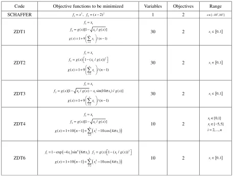
[image:5.612.78.533.138.484.2]Set the population size of all algorithms to be 50, the maximum number of iteration to be 100, and the archive size to be 100. Every algorithm runs 10 times independently. The test functions used are shown in Table 1.
Table 1. The test functions.
Code Objective functions to be minimized Variables Objectives Range
SCHAFFER 2 2
1 , 2 ( 2)
f =x f = x− 1 2 x∈ −[ 10 ,10 ]3 3
ZDT1
1 1 f =x
2 ( )[1 1/ ( )]
f =g x − x g x
2
( ) 1 9 / ( 1)
n i i
g x x n
=
= + −
∑
30 2 xi∈[ ]0,1
ZDT2
1 1 f =x
2
2 ( ) 1 (1/ ( ))
f =g x − x g x
2
( ) 1 9 / ( 1)
n
i i
g x x n
=
= + −
∑
30 2 xi∈[ ]0,1
ZDT3
1 1 f =x
2 ( )[1 1/ ( ) 1sin(10 1) / ( )]
f =g x − x g x −x πx g x
2
( ) 1 9 / ( 1)
n
i i
g x x n
=
= + −
∑
30 2 xi∈[ ]0,1
ZDT4
1 1 f =x
2 ( )[1 1/ ( )]
f =g x − x g x
( ) ( 2 ( ))
2
( ) 1 10 1 10 cos 4
n
i i
i
g x n x πx
=
= + − +∑ −
10 2
1 [0,1] [ 5,5] 2,..., i x x i n ∈ ∈ − = ZDT6
( ) 6( )
1 1 exp 41 sin 6 1
f = − − x πx 2
2 ( ) 1 ( 1/ ( ))
f =g x − x g x
( ) ( 2 ( ))
2
( ) 1 10 1 10 cos 4
n
i i
i
g x n x πx
=
= + − +∑ − 10 2 [ ]
0,1 i x∈
The front of non-inferior solution of the standard test functions are shown in Figure 1 to Figure 6 and are compared with the real Pareto front. The running time, convergence index γ and
distribution index SP are shown in the Table 2 to Table 4.
[image:5.612.328.456.528.731.2]
Figure 1. The SCHAFFER function. Figure 2. The ZDT1function.
[image:6.612.110.506.176.509.2]
Figure 5. The ZDT4 function. Figure 6. The ZDT6 function.
Table 2. The running time [second].
Algorithm CMOPSO MOEAD NSGA-II
SCHAFFER 3.3867 36.8049 26.2543
ZDT1 2.3132 21.1093 23.7799
ZDT2 2.7718 19.7723 37.7379
ZDT3 1.0341 24.3322 70.0710
ZDT4 2.3726 19.2741 36.6331
ZDT6 0.4319 17.8783 33.2695
Table 3. The convergence index γ.
Algorithm CMOPSO MOEAD NSGA-II
SCHAFFER 0.0018 1.9708 0.0029
ZDT1 0.1233 1.8550 0.3441
ZDT2 0.2277 1.9871 0.6134
ZDT3 0.0105 7.2397 0.2602
ZDT4 0.0028 5.4741 1.7583
ZDT6 0.1425 0.0457 1.4758
Table 4. The distribution index SP.
Algorithm CMOPSO MOEAD NSGA-II
SCHAFFER 0.0281 0 1.1446
ZDT1 0.0062 37.7808 0.4442
ZDT2 0.0090 0 0.4678
ZDT3 0.0160 49.7469 0.5973
ZDT4 0.0067 19.5889 0.2965
ZDT6 0.2358 0 0.5007
From Table 2, the CMOPSO converges faster than the other two algorithms. Especially, the convergence speed of the CMOPSO is 70 times that of NAGS-II for ZDT3.
For SCHAFFER, it can be seen from the tables that the performance of CMOPSO is better than the others. It can be seen from the Figure 1 that the distribution of the non-inferior solution is also better than the others.
For ZDT1, the non-inferior solution obtained by CMOPSO completely cover the real Pareto front while the other algorithms have non-coinciding parts. That is to say, CMOPSO is better distribution than other algorithms.
For ZDT2, all of the algorithms coincide with the real Pareto front, but as can be seen from the Figure 2, CMOPSO obtains the most non- inferior solution and is more uniform, covers more points. The conclusion can be confirmed from the data of distribution and convergence. That is to say, the algorithm is superior to other algorithms.
For ZDT3 and ZDT4, the algorithm covers the real Pareto front. The gap between MOEAD and the real Pareto front is more, which verifies the convergence of CMOPSO.
For MOEAD, the distribution index SP is 0, which is better than others in ZDT2, ZDT6 and
SCHAFFER. But it can be seen from the figures that the gap between MOEAD and the real Pareto front is larger. That is to say, CMOPSO is superior to MOEAD.
Based on the above analysis, the convergence and distribution of the algorithm proposed in the paper are better than that of the other two algorithms. The experiments confirm the effectiveness of CMOPSO algorithm.
Conclusion
In order to improve the convergence and distribution of multi-objective particle swarm algorithm, a chaotic particle swarm optimization algorithm based on linear inertia weight was proposed. The speed was updated with the linear decreasing inertia weight method; the searched non-inferior solution was stored in elite files and optimized with the chaotic maps. At the same time, the mutation probability is added to carry out perturbation, expand the search range, and improve the algorithm's insufficiency in local optimum. Simulation results show that the convergence and distribution of the algorithm proposed in the paper are improved.
Acknowledgement
This research was financially supported by the Science Foundation of Guizhou Province (No. [2017]1047). The authors also gratefully acknowledge the useful suggestions of the reviewers and editors.
References
[1]Zhou Liuxi, Zhang Xinghua, Li Wei, Improved multi-objective particle swarm optimization algorithm, Computer Engineering and Applications, 2009, 45(33) 38-41.
[2]Coello C A C, Lechuga M S, MOPSO: a proposal for multiple objective particle swarm optimization, 2002.
[3]Mostaghim S, Teich J, The role of ε-dominance in multi objective particle swarm optimization
methods// Evolutionary Computation, 2003, CEC '03, The 2003 Congress on, IEEE, 2003: 1764-1771 Vol. 3.
[4]Li Jing, Huang Tianmin, Chen Shangyun, Multi-objective particle swarm optimization based on angle preference for ε-Paerto domination, Journal of Xihua University (Natural Science Edition), 2018(02) 70-74[2018-04-01].
[5]Hu X, Eberhart R, Multiobjective optimization using dynamic neighborhood particle swarm optimization//Evolutionary Computation, 2002, CEC '02, Proceedings of the 2002 Congress on, IEEE, 2002 1677-1681.
[6]Agrawal S, Dashora Y, Tiwari M K, et al, Interactive Particle Swarm: A Pareto-Adaptive Metaheuristic to Multi-objective Optimization, IEEE Transactions on Systems, Man, and Cybernetics - Part A: Systems and Humans, 2008, 38(2) 258-277.
[7]Hu Wang, Gary G, Yen, Zhang Xin, Multiobjective Particles swarm optimization based on Pareto entropy, Journal of Software, 2014,25(5) 1025-1050.
[8]Liu Huihui, Research on an improved multi-objective optimization algorithm of particle swarm [J], Computer Technology and Development, 2015, 01(25), 87-90+95.
[10]Xu Xun, Study on multi-objective particle swarm optimization algorithm and its application [D], Jiang Nan University, 2014.
[11]Coello C, A comprehensive survey of evolutionary based multi-objective optimization techniques, Knowledge and Information Systems, 1999, 1(3) 269-308.
[12]Guan Hetong, Application ang implementation of cloud computing task scheduling of chaos particle swarm chicken swarm fusion optimization algorithm, Ji Lin University, 2016.
[13]Zhang W, Kwak K S, Feng C, Network selection algorithm for heterogeneous wireless networks based on multi-objective discrete particle swarm optimization, Ksii Transactions on Internet & Information Systems, 2012, 6(7) 1802-1814.
[14]Han Zhitao, Jing Yuanwei, Duan Xiaodong, Zhang Siyi, Relative degree and linearization of general nonlinear system, Control and Decision, 2006, 21(9) 1065-1067.
![Table 2. The running time [second].](https://thumb-us.123doks.com/thumbv2/123dok_us/268626.1027101/6.612.110.506.176.509/table-the-running-time-second.webp)