Test for parameter changes in generalized random coefficient autoregressive model

R E S E A R C H

Open Access

Test for parameter changes in generalized

random coefficient autoregressive model

Zhi-Wen Zhao

_{, De-Hui Wang}

_{and Cui-Xin Peng}

*_{Correspondence:}

[email protected] 1_{College of Mathematics, Jilin}

Normal University, Siping, 136000, P.R. China

Full list of author information is available at the end of the article

Abstract

In this paper, we study the problem of testing for parameter changes in generalized random coefficient autoregressive model (GRCA). The testing method is based on the monitoring scheme proposed by Naet al.(Stat. Methods Appl. 20:171-199, 2011), and the test statistic relies on the conditional least-squares estimator of an unknown parameter. Furthermore, under mild conditions, we obtain the asymptotic property of the test statistic. Some simulation studies are also conducted to investigate the finite sample performances of the proposed test.

MSC: Primary 62M10; secondary 91B62

Keywords: monitoring parameter changes; conditional least-squares estimation; asymptotic variance; generalized random coefficient autoregressive model

1 Introduction

Consider the following one-order generalized random coefficient autoregressive model (GRCA()):

Yt=tYt–+εt, t= ,±,±, . . . , (.) where (t,εt)τis a random vector withE

t εt

=φt_andVart_ε

t

=_σVφ,t σε,t ε,t σε,t

. In addition, (t,εt)τ is assumed to be independent ofFt–=σ(Yt–,Yt–, . . .).

The model (.) was first introduced by Hwang and Basawa []. Whentandεtare mu-tually independent, the model (.) becomes the random coefficient autoregressive model (RCAR), and whenVφ= , the model (.) becomes the usual autoregressive model.

Fur-thermore, the model (.) also includes the Markovian bilinear model (see,e.g., [, ]), the generalized Markovian bilinear model, and the random coefficient exponential autore-gressive model (see [] for more information) as special cases.

GRCA is designed for investigating the result of random perturbations of a dynamical system in engineering and economic data, and it has become one of the important mod-els in the nonlinear time series context. In several recent years, GRCA has been studied by many authors. For instance, Hwang and Basawa [] established the local asymptotic normality of a class of generalized random coefficient autoregressive processes. Lee [] studied the problem of testing the constancy of the coefficient. Moreover, Carrasco and Chen [] provided tractable sufficient conditions that simultaneously imply strict station-arity, finiteness of higher-order moments, andβ-mixing with geometric decay rates. In this paper, we consider the problem of testing for parameter changes in GRCA.

The change-point problem has a long history and began with i.i.d. samples (see,e.g., [– ]). Observing that time series often suffer from structural changes, statisticians started the study of the change-point problem for economic time series models (see,e.g., [, ]). Recently, the change-point problem has become very popular in economic time series. Lee and Park [] considered the monitoring process in time series regression models with nonstationary regressors. Gombay and Serban [] proposed sequential tests to detect an abrupt change in any parameter, or in any collection of parameters of an autoregressive time series model. By using the cumulative sum test, Kang and Lee [] studied the prob-lem of testing for a parameter change in a first-order random coefficient integer-valued autoregressive model. Moreover, Naet al.[] also designed the monitoring procedure in general time series models and applied it to the changes of the autocovariances of linear processes, GARCH parameters, and underlying distributions.

In order to monitor the parameter changes in generalized random coefficient autore-gressive model, we employ the monitoring scheme proposed by Naet al.[]. The test statistic relies on the conditional least-squares estimator of an unknown parameter, and under mild conditions we also obtain the asymptotic property of the test statistic.

The rest of this paper is organized as follows: In Section , we introduce the methodology and the main results. Simulation results are reported in Section . A real data analysis is given in Section . Section  provides the proofs of the main results.

Throughout this paper, we denotep-dimensional standard Brown motion by{Wp(s),s≥ }. The symbols ‘→d’ and ‘→p ’ denote convergence in distribution and convergence in prob-ability, respectively, and convergence ‘almost surely’ is written as ‘a.s.’.

2 Methodology and main results

Naet al. [] proposed a monitoring scheme of detecting parameter changes for gen-eral time series models. In what follows, we will first introduce this monitoring procedure briefly, and then we give our main results.

Let{Yt}be a time series andbe unknown parameter which will be examined for the parameter constancy. We assume thatis a constant for the historical dataY,Y, . . . ,YT. Here, we wish to test the following hypotheses based on the estimatorˆTof:

H: does not change over timet>T versusH:changes at some timet>T.

We assume that, under H,ˆTis a

√

T-consistent estimator ofbased onY,Y, . . . ,YT, its asymptotic variance-covariance matrix is nonsingular and ˆTis the consistent esti-mator of based onY,Y, . . . ,YT. We can then define

τ(T) =inf

k>T:ˆ–

 

T (ˆk–ˆT)≥ 

√

Tg

k T

, (.)

whereˆk is the estimator ofat time lagk>T based onY,Y, . . . ,Yk, · denotes a norm onRp_{, andg(s) (s∈(,∞)) is a given boundary function.}

Ifτ(T) is finite, we reject H. In actual practice, if there existsk∈(T,T+q), withq=

T, T, T, T etc., such that ˆ–

 

T (ˆk–ˆT) ≥√_Tg(_Tk), then we reject H. Meanwhile,

the boundary functiongis chosen to satisfy

lim

T→∞PH τ(T) <∞

for a givenα∈(, ) and

lim

T→∞PH τ(T) <∞

= .

Further, under H, suppose that the estimatorˆk(k=T,T+ , . . .) satisfies the following conditions:

(A) ˆkcan be decomposed as

ˆ

k=+

 k

k

t=

lt+k, (.)

whereis a true value ofunderH,{lt = (lt, . . . ,lpt)τ,t≥}is a sequence of

p-dimensional random vectors andk= (k, . . . ,pk)τ are negligible terms.

(A) There exists ap-dimensional standard Brownian motion{Wp(s),s≥}such that, for some <λ<_,

k

t=

lt– –



_{Wp(k) =Ok}λ _{a.s. (.)}

(A) For each≤i≤p,

√

Tsup_k≥T|i,k|=op().

Remark  Condition (A) holds for zero mean stationary martingale difference sequence

{lt,t≥}and at this point =E(llτ) (see [, ]).

Based on the above conditions, we have the following lemmas.

Lemma . Suppose that(A)-(A)hold.If g(s) =cg(s),s∈(,∞),c is a positive constant

and gis a given continuous real-valued function withinfs∈(,∞)g(s) > ,then

lim

T→∞PH τ(T) <∞

=P Wp(s) –sWp()≥sg(s)for some s> 

=P Wp(s)≥g

/( –s)for some <s< 

=P

sup s∈(,)

Wp(s) g(/( –s))

≥c

.

Particularly,if g(s) =c,then

lim

T→∞PH τ(T) <∞

=Psup s∈(,)

Wp(s)≥c

.

Lemma . is due to Naet al.[]. Moreover, (A)-(A) and the consistency of ˆT indi-cate that

[Ts]

√

T ˆ

–_

T (θˆ[Ts]–θˆT) w

→Wp(s) –sWp(), s∈[,∞)

Lemma . Suppose that(A)-(A)hold.If g(s) =

s–

s (e+ln( s

s–)),s∈(,∞)and · ∞

is the maximum norm,then

lim

T→∞PH τ(T) <∞

=P Wp(s) –sWp()_∞≥sg(s)for some s> 

=  – –   –(e) +eφ(e)p,

where e is a constant,φanddenote the standard normal density and distribution func-tions,respectively.

Below, we use the above method to detect parameter changes in the model (.). Suppose thatσ

ε,t=σε, ,σε,t=σε,,Vφ,t=Vφ,,t= , , . . . . Moreover, we assume thatφt=φfor

t= , . . . ,T. Consider the following hypothesis test:

H: φt=φ,t>TversusH:φtchanges at somet>T.

Before we state our main results, we list some regular conditions used in this paper.

(C) The distributions oftandεtare absolutely continuous with respect to the Lebesgue

measure onR_{and their densities are strictly positive on some neighborhood of .} (C) θ=φ+Vφ,< .

(C) E(t) < andE(εt) <∞.

Remark  It is shown by Theorem . of Hwang and Basawa [] that, under (C),{Yt,t≥}

is stationary and ergodic.

In order to establish the test statistic we need to obtain the consistent estimator of pa-rameterφunder H. Below we further assume that conditions (C)-(C) hold. Based on

the recorded data{Y, . . . ,Yk}, the conditional least-squares estimatorφˆkofφis obtained

by minimizing

S= k

t=

Yt–E(Yt|Yt–)



with respect toφ. Substituting E(Yt|Yt–) =φYt– inSand solvingdS/dφ=  forφ, we

obtain

ˆ

φk= _k

t=

Yt–Yt–

– _k

t=

YtYt–

.

Under the conditions (C) and (C), the estimatorφˆkis consistent and asymptotically nor-mal, and its asymptotic varianceJ=σ_ε,–( –θ)(σε, EY+ σε,EY+ (θ–φ)EY) (see

Hwang and Basawa []).

We now consider an estimate ofϒ. A conditional least-squares estimatorϒˆkofϒcan be obtained by minimizing

Q(ϒ) = k

t=

Y_t–EY_t|Yt–

 = k t=

Y_t–N_tτϒ,

whereNt= (Yt–, , Yt–)τ. SolvingdQ/dϒ=  forϒ, we obtain

ˆ

ϒk= _k

t=

NtNtτ –_k

t=

Y_tNt.

The following lemma indicates thatϒˆkis the consistent estimator ofϒ.

Lemma . Suppose that(C)and(C)hold.Then,underH,we have

ˆ

ϒk a.s.

→ϒ. (.)

After obtaining the consistent estimator ofφandJ, we can establish the following test

statistics:

τ(T) =inf

k>T:ˆJ–

 

T (φˆk–φˆT)≥  √ Tg k T . (.)

For the test statisticsτ(T), we have the following results.

Theorem . Suppose that(C)-(C)hold.

(i) Ifg(s) =cg(s),s∈(,∞),cis a positive constant,andgis a given continuous

real-valued function withinfs∈(,∞)g(s) > ,then

lim

T→∞PH τ(T) <∞

=P

sup s∈(,)

W(s)

g(/( –s))≥

c

.

Particularly,ifg(s) =cand · = · ,then

lim

T→∞PH τ(T) <∞

=P

sup s∈(,)

W(s)≥c

.

(ii) Ifg(s) =

s–

s (e+ln( s

s–)),s∈(,∞),and · = · ∞,then

lim

T→∞PH τ(T) <∞

=  – (e) + eφ(e).

Remark  Ifg(s) =cand · = · , we have

τ(T) =inf

k>T:ˆJ–

 

T (φˆk–φˆT)_≥ c √ T =inf

k>T:ˆJ–

 

T (φˆk–φˆT)≥ c

√

T

=inf k>T:TJˆ_T–(φˆk–φˆT)≥c

By (i) of Theorem ., we can determine the constantcfor any significance levelα∈(, ). In fact, sincelimT→∞PH{τ(T) <∞}=P{sups∈(,)|W(s)| ≥c(α)}=α, wherec(α) is the

 –αquantile point ofsup_{s∈(,)}|W(s)|, we thus havec=c(α). Whenp= , we havec= .

forα= .. Moreover, ifg(s) =

s–

s (e+ln( s

s–)),s∈(,∞), and · = · ∞, then when

p= , we havee_{= . for the nominal levelα= ..}

3 Simulation results

In this section, we evaluate the performance of the monitoring test through a simulation study.

Consider the following model:

Yt= (φ+αεt)Yt–+εt, (.)

where{εt}is i.i.d. normally distributed with mean  and variance .

We compare the performance of testing methods (i) and (ii) in Theorem .. For the testing method (i), we takeg(s) =cand · = · . In the actual simulation, we reject

Hif there existsk∈(T,T +q) such thatˆJ –_

T (φˆk–φˆT) ≥ √_Tg(_Tk), where the horizon q= T, T, Tand T, andT= , , ,  and ,. In each simulation, , observations are discarded to remove initialization effects and a repetition number of , is utilized.

In the first simulation, we calculate the probability of rejecting the null hypothesis when it is true at the nominal levelα= .. The results of the simulations are presented in Table , and the figures in parentheses are those for a constant function test.

From Table , we see that the test with the boundary function in (ii) of Theorem . has superiority over that with the constant boundary function. We can also see that the empirical sizes of these two tests tend to decrease as the historical sample sizeTincreases and increase asqincreases. But even ifTis small orqis large, the empirical sizes of these two testing methods are still very close to the nominal level.

The second simulation study is designed to examine the power. We calculate the proba-bility of rejecting the null hypothesis when the alternative hypothesis is true at the nominal levelα= .. To do this, we consider the alternative hypotheses as follows:

H: A change occurs fromφt= .,α= .toφt= .,α= .;

˜

H: A change occurs fromφt= .,α= .toφt= .,α= ..

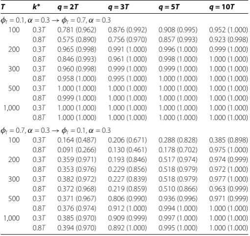
In all cases, the changes are assumed to occur atk∗= .Tandk∗= .T. The results of the simulations are presented in Table , and the figures in parentheses are those for the constant function test.

Table 1 Empirical sizes

φt T q= 2T q= 3T q= 5T q= 10T

0.1 100 0.084 (0.179) 0.084 (0.207) 0.070 (0.255) 0.096 (0.285) 200 0.050 (0.167) 0.061 (0.181) 0.046 (0.228) 0.049 (0.245) 300 0.061 (0.162) 0.057 (0.207) 0.056 (0.229) 0.053 (0.257) 500 0.071 (0.139) 0.050 (0.184) 0.054 (0.242) 0.059 (0.258) 1,000 0.056 (0.153) 0.058 (0.185) 0.055 (0.224) 0.065 (0.300)

0.3 100 0.085 (0.170) 0.097 (0.235) 0.090 (0.264) 0.103 (0.261) 200 0.088 (0.149) 0.071 (0.202) 0.054 (0.216) 0.078 (0.253) 300 0.071 (0.156) 0.060 (0.196) 0.069 (0.229) 0.069 (0.266) 500 0.065 (0.159) 0.072 (0.192) 0.070 (0.223) 0.073 (0.272) 1,000 0.077 (0.169) 0.062 (0.195) 0.065 (0.250) 0.069 (0.260)

0.5 100 0.090 (0.160) 0.077 (0.174) 0.109 (0.223) 0.101 (0.234) 200 0.086 (0.121) 0.082 (0.159) 0.070 (0.182) 0.078 (0.198) 300 0.087 (0.149) 0.077 (0.136) 0.066 (0.174) 0.060 (0.208) 500 0.071 (0.137) 0.069 (0.142) 0.063 (0.188) 0.073 (0.203) 1,000 0.073 (0.118) 0.064 (0.151) 0.069 (0.186) 0.069 (0.220)

0.7 100 0.078 (0.138) 0.055 (0.092) 0.111 (0.184) 0.094 (0.192) 200 0.063 (0.098) 0.073 (0.090) 0.065 (0.097) 0.058 (0.115) 300 0.076 (0.096) 0.064 (0.083) 0.057 (0.110) 0.054 (0.091) 500 0.052 (0.078) 0.055 (0.089) 0.067 (0.108) 0.056 (0.117) 1,000 0.041 (0.081) 0.069 (0.081) 0.049 (0.117) 0.063 (0.111)

0.9 100 0.067 (0.100) 0.049 (0.063) 0.078 (0.117) 0.098 (0.161) 200 0.036 (0.042) 0.041 (0.052) 0.049 (0.071) 0.041 (0.085) 300 0.037 (0.060) 0.044 (0.057) 0.051 (0.060) 0.044 (0.069) 500 0.046 (0.056) 0.038 (0.068) 0.032 (0.064) 0.049 (0.074) 1,000 0.033 (0.042) 0.047 (0.063) 0.039 (0.065) 0.035 (0.081)

Table 2 Empirical powers

T k∗ q= 2T q= 3T q= 5T q= 10T

φt= 0.1,α= 0.3→φt= 0.7,α= 0.3

100 0.3T 0.781 (0.962) 0.876 (0.992) 0.908 (0.995) 0.952 (1.000) 0.8T 0.575 (0.890) 0.756 (0.970) 0.857 (0.993) 0.923 (0.998) 200 0.3T 0.965 (0.998) 0.991 (1.000) 0.996 (1.000) 0.999 (1.000) 0.8T 0.846 (0.993) 0.961 (1.000) 0.998 (1.000) 1.000 (1.000) 300 0.3T 0.960 (0.998) 0.999 (1.000) 0.999 (1.000) 1.000 (1.000) 0.8T 0.958 (1.000) 0.995 (1.000) 1.000 (1.000) 1.000 (1.000) 500 0.3T 1.000 (1.000) 1.000 (1.000) 1.000 (1.000) 1.000 (1.000) 0.8T 0.999 (1.000) 1.000 (1.000) 1.000 (1.000) 1.000 (1.000) 1,000 0.3T 1.000 (1.000) 1.000 (1.000) 1.000 (1.000) 1.000 (1.000) 0.8T 1.000 (1.000) 1.000 (1.000) 1.000 (1.000) 1.000 (1.000)

φt= 0.7,α= 0.3→φt= 0.1,α= 0.3

100 0.3T 0.164 (0.487) 0.206 (0.671) 0.288 (0.828) 0.385 (0.898) 0.8T 0.091 (0.266) 0.130 (0.461) 0.178 (0.702) 0.975 (1.000) 200 0.3T 0.359 (0.971) 0.193 (0.846) 0.517 (0.974) 0.974 (0.999) 0.8T 0.353 (0.976) 0.229 (0.856) 0.518 (0.979) 0.972 (1.000) 300 0.3T 0.382 (0.972) 0.227 (0.839) 0.518 (0.979) 0.977 (1.000) 0.8T 0.372 (0.968) 0.219 (0.859) 0.510 (0.866) 0.963 (0.999) 500 0.3T 0.371 (0.967) 0.806 (0.990) 0.936 (0.996) 0.971 (0.999) 0.8T 0.376 (0.974) 0.912 (1.000) 0.994 (1.000) 1.000 (1.000) 1,000 0.3T 0.385 (0.970) 0.909 (0.999) 0.997 (1.000) 1.000 (1.000) 0.8T 0.394 (0.970) 0.892 (1.000) 0.995 (1.000) 1.000 (1.000)

4 Real data analysis

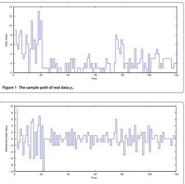
We mainly pay attention to drugs data series. The data are available on-line at the fore-casting principles site (http://www.forefore-castingprinciples.com/index.php?option=com_ content&view=article&id=&Itemid=). An observation of the time series represents a count of drugs reported in the police car beat in Pittsburgh, during one month. The data consist of  observations, starting in January  and ending in December . The data are denotedy,y, . . . ,y. Figure  is the sample path plot for the real datayt,

t= , , . . . , .

The sample path plot reveals nonstationarity. Therefore, letxt =yt–yt–. The sample

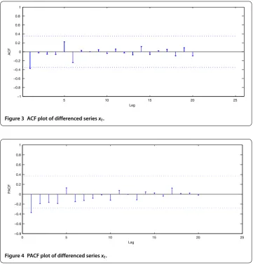
path plot, the autocorrelation function (ACF), and the partial autocorrelation function (PACF) for the differenced seriesxtis given in Figures , , and , respectively. From Fig-ure , we can see thatxtis from a stationary series. From Figures  and , we can see that xtmay come from anGRCA() process. Therefore, we consider a model of the data series xt by using the following:

xt= (φ+αεt)xt–+εt, (.)

where{εt}is for i.i.d. random variables.

We assume thatφ is a constant for the historical datax,x, . . . ,x. Then we test the

following hypotheses:

Figure 1 The sample path of real datayt.

Figure 3 ACF plot of differenced seriesxt.

Figure 4 PACF plot of differenced seriesxt.

H: φdoes not change over timet> versusH:φchanges at some timet> .

Based on the historical datax,x, . . . ,x, testing methods (i) and (ii) in Theorem .

both accept the null hypothesis. That is to say, φ does not change over time t> . Further, we use the data x,x, . . . ,x to estimate the unknown parameters φ andα,

respectively. Therefore, we can model the data x,x, . . . ,x by using the model xt = (–. + .εt)xt–+εt, where{εt}is for i.i.d. random variables.

5 Proofs of the main results

In order to prove the main results, we need some auxiliary lemmas.

Lemma . Suppose that (C)-(C)hold. Then, under H, one-order generalized

ran-dom coefficient autoregressive model(.)isβ-mixing with geometric decaying order and EY

t <∞.

Proof The proof can be found in Carrasco and Chen [].

Lemma . Suppose that(C)-(C)hold.Then,underH,for the one-order generalized

for any <d< ,

lim sup k→∞

|k

t=(Ytd–EYtd)|

klog logk ≤M a.s.

Proof This lemma can be proved by Lemma . and Theorem  in Kuelbs and Philipp

[].

Lemma . Let{Yi,i≥}be a stationary ergodic stochastic sequence with E(Yi|Y,Y,

. . . ,Yi–) = a.s.for all i≥and EY= .Thenlim supn→∞ n

i=

Yi (nlog logn)

= a.s.

Proof The proof can be found in Stout [].

Proof of Lemma. Note that

 k k t=

NtNtτ

(ϒˆk–ϒ) =  k k t= Y_t–Nτ

tϒ

Nt. (.)

By the ergodic theorem, we have

 k

k

t=

NtNtτ

a.s.

→ENNτ

(.) and  k k t=

Y_t–N_tτϒNt

a.s.

→. (.)

These, together with (.), imply thatϒˆk

a.s.

→ϒ, and thus the proof of Lemma . is

com-plete.

Proof of Theorem. We apply Lemma . to prove Theorem ..

Firstly we decomposeφˆkinto the sum of martingale differences and a negligible term. Note that

ˆ

φk= k

t=YtYt–

k

t=Yt–Yt–

=φ+

k t=YtYt–

k

t=Yt–Yt–

–φ=φ+

k

t=(Yt–φYt–)Yt–

k

t=Yt–Yt–

=φ+ 

k k

t=(Yt–φYt–)Yt–

EY_ +



k k

t=(Yt–φYt–)Yt– 

k k

t=Yt–Yt–

–



k k

t=(Yt–φYt–)Yt–

EY 

=φ+ 

k n

t=(Yt–φYt–)Yt–

EY  –  k k t=

Yt–Yt–

–

EY_–

×  k k t=

Yt–Yt––EY

 k k t=

(Yt–φYt–)Yt–

Next, we verify that they meet the conditions of Lemma .. Observe that (EY

) –

{(Yt–φYt–)Yt–,t≥} is a sequence of mean zero stationary

martingale difference. Thus, there exists a -dimensional standard Brownian motion

{W(s),s≥}such that, for some  <λ<_,

k

t=

EY_–(Yt–φYt–)Yt––J– 

_{W(k) =Ok}λ _{a.s. (.)}

In what follows, we prove that

√

Tsup k≥T

(_kk_t=Yt–Yt––EY)k k

t=(Yt–φYt–)Yt–

(_kk_t=Yt–Yt–)EY

=op(). (.)

By Lemma ., we have

lim sup k→∞



(klog logk)

k

i=

(Yt–φYt–)Yt–=

E(Yt–φYt–)Yt– a.s. (.)

From Lemma . we know that there exists a positive constantMsuch that, for any  <

d< ,

lim sup k→∞

|k

t=(Ytd–EYtd)|

klog logk ≤M a.s., (.)

from which, together with (.), we have

√

k(



k k

t=Yt–Yt––EY)k k

t=(Yt–φYt–)Yt–

(_kk_t=Yt–Yt–)EY

a.s.

→ ask→ ∞. (.)

Further, note that

√

Tsup k≥T

(_kk_t=Yt–Yt––EY)k k

t=(Yt–φYt–)Yt–

(

k k

t=Yt–Yt–)EY

≤sup k≥T

√

k(



k k

t=Yt–Yt––EY)k k

t=(Yt–φYt–)Yt–

(_kk_t=Yt–Yt–)EY

. (.)

By (.), we prove (.). Thus, by Lemma ., we prove Theorem ..

Competing interests

The authors declare that they have no competing interests.

Authors’ contributions

All authors contributed equally to the writing of this paper. All authors read and approved the final manuscript.

Author details

1_{College of Mathematics, Jilin Normal University, Siping, 136000, P.R. China.}2_{College of Mathematics, Jilin University,}

Acknowledgements

This work is supported by National Natural Science Foundation of China (Nos. 11271155, 11001105, 11071126, 10926156, 11071269), Specialized Research Fund for the Doctoral Program of Higher Education (Nos. 20110061110003,

20090061120037), Scientific Research Fund of Jilin University (Nos. 201100011, 200903278), the Science and Technology Development Program of Jilin Province (201201082), Jilin Province Social Science Fund (2012B115) and Jilin Province Natural Science Foundation (20101596, 20130101066JC).

Received: 9 March 2014 Accepted: 25 July 2014 Published:21 Aug 2014

References

1. Hwang, SY, Basawa, IV: Parameter estimation for generalized random coefficient autoregressive processes. J. Stat. Plan. Inference68, 323-327 (1998)

2. Tong, H: A note on a Markov bilinear stochastic process in discrete time. J. Time Ser. Anal.2, 279-284 (1981) 3. Feigin, PD, Tweedie, RL: Random coefficient autoregressive processes: a Markov chain analysis of stationarity and

finiteness of moments. J. Time Ser. Anal.6, 1-14 (1985)

4. Hwang, SY, Basawa, IV: Asymptotic optimal inference for a class of nonlinear time series models. Stoch. Process. Appl.

46, 91-113 (1993)

5. Hwang, SY, Basawa, IV: The local asymptotic normality of a class of generalized random coefficient autoregressive processes. Stat. Probab. Lett.34, 165-170 (1997)

6. Lee, S: Coefficient constancy test in a random coefficient autoregressive model. J. Stat. Plan. Inference74, 93-101 (1998)

7. Carrasco, M, Chen, X:β-Mixing and moment properties of RCA models with application to GARCH(p,q). C. R. Acad. Sci., Sér. I Math.331, 85-90 (2000)

8. Page, ES: Continuous inspection schemes. Biometrika41, 100-114 (1954)

9. Page, ES: A test for a change in a parameter occurring at an unknown point. Biometrika42, 523-527 (1955) 10. Page, ES: On problems in which a change in parameter occurs at an unknown point. Biometrika44, 248-252 (1957) 11. Hinkley, DV: Inference about the change-point from cumulative sum tests. Biometrika58, 509-523 (1971) 12. Brown, RL, Durbin, J, Evans, JM: Techniques for testing the constancy of regression relationships over time. J. R. Stat.

Soc., Ser. B37, 149-163 (1975)

13. Inclan, C, Tiao, GC: Use of cumulative sums of squares for retrospective detection of changes of variances. J. Am. Stat. Assoc.89, 913-923 (1994)

14. Wichern, DW, Miller, RB, Hsu, DA: Changes of variance in first-order autoregressive time series models - with an application. J. R. Stat. Soc., Ser. C25, 248-256 (1976)

15. Lee, S, Ha, J, Na, O, Na, S: The cusum test for parameter change in time series models. Scand. J. Stat.30, 781-796 (2003) 16. Lee, S, Park, S: The monitoring test for the stability of regression models with nonstationary regressors. Econ. Lett.

105, 250-252 (2009)

17. Gombay, E, Serban, D: Monitoring parameter change in AR(p) time series models. J. Multivar. Anal.100, 715-725 (2009)

18. Kang, J, Lee, S: Parameter change test for random coefficient integer-valued autoregressive processes with application to polio data analysis. J. Time Ser. Anal.30, 239-258 (2009)

19. Na, O, Lee, J, Lee, S: Monitoring parameter change in time series models. Stat. Methods Appl.20, 171-199 (2011) 20. Eberlein, E: On strong invariance principles under dependence assumptions. Ann. Probab.14, 260-270 (1986) 21. Kuelbs, J, Philipp, W: Almost sure invariance principles for partial sums of mixingB-valued random variables. Ann.

Probab.8, 1003-1036 (1980)

22. Chu, CSJ, Stinchcombe, M, White, H: Monitoring structural change. Econometrica64, 1045-1065 (1996) 23. Kuelbs, J, Philipp, W: Almost sure invariance principles for partial sums of mixingB-valued random variables. Ann.

Probab.8, 1003-1036 (1980)

24. Stout, WF: The Hartman-Wintner law of the iterated logarithm for martingales. Ann. Math. Stat.41, 2158-2160 (1970)

10.1186/1029-242X-2014-309