2019 International Conference on Applied Mathematics, Modeling, Simulation and Optimization (AMMSO 2019) ISBN: 978-1-60595-631-2
Data Assimilation Algorithm for Remaining Useful Life Prediction of
Aircraft Engine
Zi-min CAI, Ru-sheng JU, Xu XIE and Song WANG
National University of Defense Technology, Changsha, China
Keywords:Data assimilation, Aircraft engine, Particle filter, Remaining useful life.
Abstract. It’s a challenge to predict the remaining useful life of the aeroengine. The performance
degradation of aircraft engines involves many parameters, so it is difficult to establish an accurate physical failure model. However, with time running, its performance degradation will be reflected in the change of monitoring parameters. In this paper, a kind of remaining life prediction algorithm based on data assimilation was proposed. The real-time data collected during the operation was used to predict the change trend of engine parameters, and then the remaining life of the engine was further predicted. Experiments show that the prediction method of engine remaining life based on data assimilation has better effects, which provides a new idea and method for engine remaining life prediction.
Introduction
At present, aviation industry is in a period of vigorous development, but there are still problems in equipment maintenance and maintenance costs. The aeroengine is the core power source of the satellite, with high safety and reliability requirements, and its high costs of design, manufacturing and maintenance [1].
Remaining Useful Life (RUL) mainly refers to the remaining service life after a period of operation of the system, accurately predicting the remaining useful life of the system, which can greatly reduce the loss caused by system downtime and improve the reliable operation of the system [2]. Residual life prediction is the key and difficult point of Prognostic and Health Management (PHM) technology [3]. If the remaining life of equipment can be estimated in the early stages of equipment degradation, especially when significant hazards have not been caused, and on this basis, the best time to maintain the equipment can be determined, not only can the safety be greatly improved and failures be avoided, but also the downtime can be can be effectively reduced, the maintenance cycle can be shortened, and the maintenance process can be simplified, thereby saving maintenance costs.
Related Researches on Traditional Life Prediction Methods
In the field of residual life prediction, the predecessors have done a lot of research work. Jardine et al.[4]divided the existing residual life prediction methods into three categories, namely the prediction method based on failure mechanism model and the prediction method based on artificial intelligence, and the prediction method based on statistical data. Pecht et al. [5] combined the prediction method based on statistical data with the method based on artificial intelligence, i.e., data-driven prediction method.
Method Based on Failure Mechanism Model
The prediction method based on the failure mechanism model is a method which establishes a corresponding model by in-depth analysis of the failure physics and chemical reaction law of the product based on the failure principle of the equipment.
Data-driven Prediction Method
Data-driven prediction method includes the prediction method based on artificial intelligence and the prediction methods based on statistical data.
Among them, the method based on artificial intelligence mainly relies on machine learning, and attempts to understand the trend of equipment degradation from a large number of historical data containing fault labels and process degradation characteristic quantity to achieve residual life prediction [6]. However, this method usually requires a sufficient amount of historical failure data as a support, but as the reliability of the equipment continues to increase, it is often difficult to obtain a large amount of failure data or it will spend huge costs. In contrast, the life prediction method based on statistical data obtains the probability distribution of the residual life by establishing a mathematical statistical model of equipment performance degradation, which not only predicts the average residual life, but also the impact from uncertainty is taken into account, so it has certain advantages.
Shortcomings of the Traditional RUL Method
In the life prediction of aeroengine, the traditional RUL method has certain deficiencies.
The life prediction method based on the failure mechanism model needs to construct an accurate physical model for the target to be measured, and master the failure mechanism of the engine in detail. However, the physical model of the aeroengine is very complicated, and the parameters involved in the modeling are many, and it is very difficult to construct the model, thus, the method based on the failure mechanism model is not applicable to aeroengine.
Aeroengine has high reliability, have few failure data, and cannot provide a large amount of fault data. Therefore, the life prediction method based on historical failure data is not suitable for high-precision equipment such as aeroengine.
Currently, the life prediction of aeroengine is primarily based on statistical data-driven method to establish a mathematical statistical model of product degradation. However, this method currently has the following two shortcomings:
In the prediction method, if the model parameters can be adjusted according to the individual differences of the aeroengine, and the model is corrected in time with real-time data, the accuracy of the life prediction can be improved to some extent.
For these two shortcomings, data assimilation is an ideal solution. Through data assimilation, the real-time data monitored during engine operation can be reasonably utilized, and the parameters of the model can be adjusted in time to reduce the cumulative error that may exist during the operation of the model. At the same time, individual differences can be distinguished according to the data of each engine so that the prediction is more accurate.
Related Researches of Data Assimilation
Data assimilation refers to the method of merging new observation data and estimating the state of the system during the dynamic operation of the numerical model based on the spatial and temporal distribution of the data and the error of the observation field and the background field [7]. Its purpose is to combine the observation data generated during the operation of the system to adjust the parameters in the model in real time to reduce the cumulative error and make the result closer to the real data.
Common methods for data assimilation include particle filter and Kalman filter. Kalman filter refers to the linear system, while particle filter is better for nonlinear system. As for aerongine , particle filter is obviously better[8].
probability distribution is modified to make the approximation closer to the true system state probability distribution.
Assume a nonlinear system[9]:
1 ( )
k k k
x f x (1)
1 ( )
k k k
z h x (2) Where xk is the state of system at the time k, zk is the observations at the time k, f is a possibly nonlinear function of the state xk, h is a possibly nonlinear function of the observations, and k and k are the Gaussian white noise sequence.
The main idea of the particle filter algorithm is described in mathematical language as [10]: For the stationary dynamic time-varying system, assuming that the posterior probability density of the system at time k-1 is p x( k1|zk1), N random sample points are selected according to a certain principle, and after obtaining the measurement information at time k, after the state update and time update process, the posterior probability density of N particles is approximated as p x( k|zk). As the number of particles increases, the probability density function of the particle gradually approaches the probability density function of the state, and the estimation of the particle filter achieves the effect of optimal Bayesian estimation.
To more conveniently present the algorithm details,
0:
1
, N
i i
k k i x w
is defined to represent a
collection of samples (or particles), where,
x0:ik,i0,...,N
refers to the state value of the particles,
w iki, 0,...,N
refers to the weight values corresponding to the particles and satisfy the condition:1 N i k i w
, and N refers to the number of particles.Assuming that the prior distribution p x( 0:ik1|z1:k1) is known, and N samples have been obtained from the system model, the approximate posterior distribution can be expressed as
0: 1: 0: 0:
1
( | ) ( )
N
i i
k k k k k
i
p x z w x x
(3) Where (*) refers to the dirac delta function.Since it is difficult to sample directly from the posterior distribution, the importance sampling technique can be used to sample the particles from the importance distribution. The particle weights are updated according to the method of importance sampling:
0: 1: 0: 1:
( | )
( | )
i
i k k
k i
k k
p x z
w
q x z
(4) The importance distribution q x( 0:k|zk) is decomposed as
0: 1: 0: 1 0: 1 1
( k| k) ( k| k , k) ( k | k )
q x z q x x z q x z (5) To derive the equation for weight update, p x( 0:k1|z1:k1), (p zk|xk) and p x( k|xk1) are used to express p x( 0:k|z1:k):
1
0: 1: 0: 1 1: 1
1: 1 ( | ) ( ( )) ( | ) ( | ) ( | )
k k k k
k k k k
k k
p z x p x x
p x z p x z
1 1 0: 1 ( | ) ( | ) ( | , )
i i i
i i k k k k
k k i i
k k k
p z x p x x
w w
q x x z (7)
Assuming the system is a Markov process, the weight update equation can be further simplified as:
1 1
1
( | ) ( | ) ( | , )
i i i
i i k k k k
k k i i
k k k
p z x p x x
w w
q x x z
(8) If the state transition distribution is used as the importance distribution:
1 1
( ki | ki , k) ( ik| ik )
q x x z q x x (9) a simplified expression of the weight update can be gained:
1 ( | )
i i i
k k k k
w w p z x (10) As the number of iteration increases, there are only a few particles whose weights play a significant role, while the weights of other particles are almost reduced to zero, which causes the problem of particle degradation. Resampling techniques are used to effectively avoid this problem. Its approach is to remove low-weight particles and copy high-weight particles to renormalize the distribution, and to reset the weights of all particles according to the specific algorithm. This is the resampling algorithm for standard particle filtering .
Through the above steps, the basic particle filtering process can be realized. The particle filter algorithm converts the integral problem into a weighted summation problem, which greatly simplifies the operation so that the filtering process is easier. Particle filter is widely used in many fields due to its flexibility and applicability. Especially for nonlinear non-Gaussian problems, particle filter method has a good effect.
Life Prediction Method Based on Particle Filtering
Health Status of Engine
The health status of an aeroengine cannot be directly observed, but as operating time increases, its performance degradation is reflected in changes in monitoring parameters[11]. These parameters mainly include gas path performance monitoring parameters, lubricating oil monitoring parameters and vibration monitoring parameters.
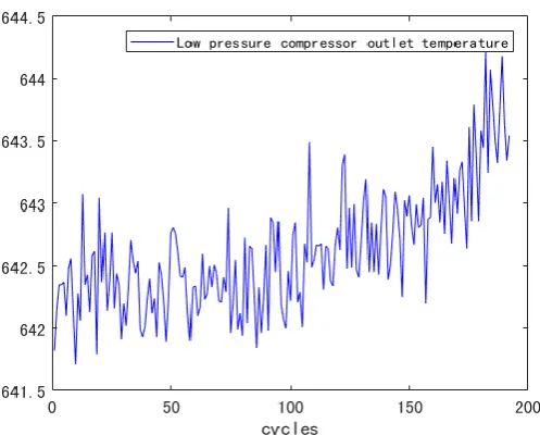
The engine performance degradation process contains a large number of accurate and reliable information closely related to engine life. Therefore, based on the change of engine performance parameters, by virtue of the performance degradation data, the degradation process of engine function is studied. When the performance degradation parameter exceeds the failure threshold, that is, a failure occurs, the residual life of the engine can be estimated.
Figure 1. The change of parameter with engine operation.
The data show that when the temperature rises to a certain extent, the engine cannot maintain normal operation and the life is terminated. Therefore, if the degradation trend of these parameters can be accurately predicted, it is possible to understand the health status of the engine and then the residual life of the engine is further predicted.
Parameter Prediction Function Based on Particle Filter
Taking a engine parameter, the temperature of high-pressure compressor outlet , as an example to carry out the parameter prediction experiment.
Polynomial functions have the ability to approximate arbitrary nonlinear functions . From the C-MAPSS data set, it can be found that there is a nonlinear relationship between the the pressure of the high pressure compressor outlet and cycles, so the polynomial function is selected for fitting. According to the fitting of data in the training set, it is found that the relationship between the pressure ofhigh-pressure compressor outlet and cycles can be expressed by the following formula:
2
* *
ya n b nc (11) Where y refers to the engine parameter, the pressure ofhigh-pressure compressor outlet, n refers to the numbers of the cycles ; a, b, and c are the parameters to be tested, respectively, containing noise. The noise is Gaussian white noise with a mean of 0 and unknown variance. According to the formula, the state of the prediction model can be given:
T
( ) [ ( ) ( ) ( )]
x k a k b k c k
(12) Then the equation of state is:
( 1) ( ) , ~ (0, )
x k x k w w N (13) The observation equation is:
2
( ) [ 1] ( ) ( )
z k k k x k v k (14) Where, ( )v k is Gaussian white noise with a mean of 0 and a variance of v.
Tracking Experiment
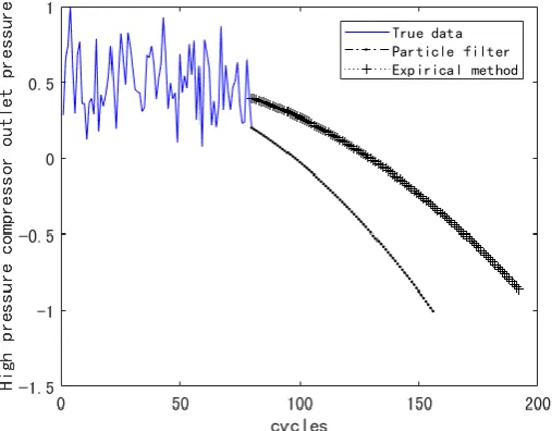
Figure 2. Estimated data based on particle filter. Figure 3. True data in the experiment.
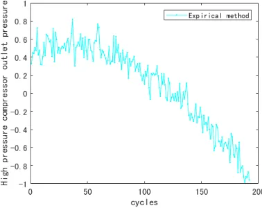
[image:6.595.89.498.76.233.2]In order to better observe the tracking effect based on the particle filter, a contrast experiment is arranged. The control group used an empirical method based on historical data statistics, and its tracking effect is shown in Figure 4:
Figure 4. Estimated data based on empirical method.
The tracking error of the two groups of tests is shown in Figure 5:
[image:6.595.197.386.305.455.2]
a. tracking error based on particle filter b. tracking error based on empirical method Figure 5. Tracking error of the two groups of tests.
In order to more intuitively compare the tracking effect, the average tracking error En is defined as follow:
s r
y y En
n
[image:6.595.87.508.497.663.2]Table 1. The average tracking error for both experiments.
Particle filter Estimated data
En 0.0421 0.1707
In the tracking test, in general, the method based on particle filtering is better than the empirical method based on historical data in tracking effect. At the beginning of engine operation, the empirical method is closer to the true value. With the increase of the number of turns, the tracking effect of the method based on particle filtering is getting better and better, and the error is getting smaller and smaller, while the errors of empirical method accumulate, resulting in poor tracking effect because it does not dynamically adjust parameters according to real-time data. Experiments show that the particle filter method has good adjustment characteristics and stability.
Prediction Experiment
The data of the No. 1 engine in the C-MAPSS data set were selected for experiment prediction. The experimental steps based on historical data are as follows:
According to the first 80 sets of data given in the sample, the parameters a, b, c are fitted, and then the parameters are predicted according to the fitted state equation.
The prediction experiment steps based on the particle filtering method are as follows:
(1) Performing particle filtering based on the first 80 sets of data in the sample is to dynamically adjust the parameters a, b, c in the state equation according to the real data;
[image:7.595.165.419.392.590.2](2) After the 80th set of data, the values of the a, b, and c parameters obtained by the particle filtering in the earlier stage are used to predict the future trend of the parameter change. The result is shown in Figure 6:
Figure 6. Prediction Results of remaining useful life.
The summary of the sample data and other literature found that when the total pressure of the high pressure compressor outlet is close to -0.9 (after normalization), the engine enters the failure domain , that is, the engine stops working.
According to the defined failure domain, during the experiment process, when the predicted total pressure of the high pressure compressor outlet is lower than -0.9, the current number of turns is recorded. The result gained from here is the number of turns the engine can work normally, minus the known 80 turns, the result is the predicted residual life. In this experiment, the prediction results of the two methods are shown in Table 2:
Table 2. The prediction results.
True data Particle filter empirical method
Results of prediction/cycles —— 156 192
Remaining useful life/cycles
The prediction errors of two methods are shown as follow:
Table 4. The prediction errors of two methods.
Particle filter Empirical method
Error/cycles 15 21
As can be seen from the table, in this experiment, particle filter based prediction methods are more accurate than empirical methods based on historical data.
Summary
For the residual life prediction of aeroengine, this paper proposes a prediction method based on particle filtering. Due to the many parameters involved in the engine, it is very difficult to accurately model the performance degradation of the engine. On the other hand, the change of the monitoring parameters of the engine sensor can largely reflect the current state of the engine, so the monitoring parameters can be modeled and predicted to further estimate the residual life of the engine. The experimental results show that the prediction method based on particle filtering has good tracking performance, which can modify the parameters to be tested in the model in a real time according to real-time data, and has good stability; in addition, its prediction results of parameters are close to the true values, and the prediction results for the residual life are good. In summary, this approach method provides a new idea and way for the prediction of the residual life of aeroengine.
Acknowledgement
This research was financially supported by the National Science Foundation 61673388.
References
[1] Zhang Chunxiao, Yue Junjie , Application of an improved adaptive chaos prediction model in aero-engine performance parameters [J]. WSEAS Transactions on Mathematics, 2012, 11(2):114-124
[2] K. Medjaher, D. A. Tobon-Mejia, N. Zerhouni. Remaining useful 1ife estimation of critical components with application to bearings[J].IEEE Transactions on Reliability, 2012, 61(2): 292–302. [3] Catiuo E, Fernandez Canteli A.A general regression model for 1ifetime evaluation and predict ion[J].International Journal of Fracture, 200l, 107(2): l 17–137.
[4] Andrew K.S. Jardine, Daming Lin, Dragan Banjevic. A review on machinery diagnostics and prognostics implementing condition-based maintenance[J]. Mechanical Systems and Signal Processing, 2006, 20(7):1483-1510.
[5] N.M. Vichare, M.G. Pecht. Prognostics and health management of electronics[J]. IEEE Transactions on Components and Packaging Technologies, 2006, 29(1):222-229.
[6] Si X S, Wang W, Hu C H, et al. Remaining useful life estimation - A review on the statistical data driven approaches[J]. European Journal of Operational Research, 2011, 213(1): 1-14.
[7] Christopher K Wikle. Atmospheric Modeling, Data Assimilation, and Predictability[J]. Technometrics, 2002, 47(4):521-521.
[8] Gordon N J, Salmond D J, Smith A F M. Novel approach to nonlinear/non-Gaussian Bayesian state estimation[J]. IEE Proceedings F - Radar and Signal Processing, 2002, 140(2):107-113.
[10] J. Carpenter, P. Clifford, P. Fearnhead. Improved particle filter for nonlinear problems[J]. IEEE Proceedings-Radar Sonar and Navigation, 2002, 146(1):2-7.