Estimation of Nonparametric Multiple Regression Measurement Error Models with Validation Data

http://dx.doi.org/10.4236/ojs.2015.57080

Estimation of Nonparametric Multiple

Regression Measurement Error Models

with Validation Data

Zanhua Yin, Fang Liu

College of Mathematics and Computer Science, Gannan Normal University, Ganzhou, China

Received 3 November 2015; accepted 27 December 2015; published 30 December 2015

Copyright © 2015 by authors and Scientific Research Publishing Inc.

This work is licensed under the Creative Commons Attribution International License (CC BY).

http://creativecommons.org/licenses/by/4.0/

Abstract

In this article, we develop estimation approaches for nonparametric multiple regression mea-surement error models when both independent validation data on covariables and primary data on the response variable and surrogate covariables are available. An estimator which integrates Fourier series estimation and truncated series approximation methods is derived without any er-ror model structure assumption between the true covariables and surrogate variables. Most im-portantly, our proposed methodology can be readily extended to the case that only some of cova-riates are measured with errors with the assistance of validation data. Under mild conditions, we derive the convergence rates of the proposed estimators. The finite-sample properties of the es-timators are investigated through simulation studies.

Keywords

Ill-Posed Inverse Problem, Linear Operator, Measurement Errors, Nonparametric Regression, Validation Data

1. Introduction

We can consider the following nonparametric regression model of a scaler response Y on an explanatory variable X

( )

,

Y=g X +ε (1)

where g

( )

⋅ is assumed to be a smooth, continuous but unknown nonparametric regression function and ε is a noise variable with E

(

ε|X

)

=0 and _E

( )

ε2 _{< ∞}

inde-pendent replicates

(

W Y_i, _i

)

, 1≤ ≤i N, of

(

W Y,

)

rather than

(

X Y,

)

, where the relationship between Wi

and Xi may or may not be specified. If not, the missing information for the statistical inference will be taken

from a sample

(

W X_j, _j

)

, N+ ≤ ≤1 j N+n, of so-call validation data independent of the primary (surrogate) sample. The objective of this manuscript is to estimate the unknown function g

( )

⋅ via the surrogate data

(

)

{

,

}

1

N i i _i

Y W ₌ and the validation data

{

(

)

}

1

, N n

j j j N

X W +

= + .

A wide number of problems of similar type have attracted considerable attention in research literature over the past two decades (see, [1]-[6]). For instance, a quasi-likelihood method is intensively studied by [7]. A re-gression calibration approach is developed by [8] [9] and [10] [11] propose a method based on simulation- extrapolation (SIMEX) estimation. Other related methods include Bayesian approaches (see, [12]), semi-parametric method (see, [13][14]), empirical likelihood method (see, [15]) and the instrumental variable method (see, [16]). Unfortunately, all these work mostly assume some parametric relationships between covariates and responses. Recently, nonparametric estimators of g have been developed by [17] and [18]. [17] develops a kernel-based approach for nonparametric regression function estimation with surrogate data and validation sampling. Howev-er, his method is not applicable for model (1) since it assumes that the response but not the covariable is meas-ured with error. [18] proposes a nonparametric estimator which integrates local linear regression and Fourier transformation method when both explanatory and surrogate variable are scalars. Nonetheless, their method cannot be extended to multidimensional problems in which the explanatory variable vectors can consist of va-riables being measured with or/and without errors. For additional references and relevant topics for nonparame-tric regression models with measurement errors, ones may consult [19] and the references therein.

In practice, nonparametric estimation of g may not be an easy task since, as explained in Section 2, the rela-tion that identifies g is a Fredholm equation of the first kind, i.e.

,

Tg=m (2) which may lead to an ill-posed inverse problem. Ill-posed inverse problem related to nonparametric regression model has received considerable attention recently. [20][21] consider kernel-based estimators while [22] and [23] develop series or sieve estimators. However, their methods require an instrumental variable, and assume that the explanatory variable X is directly observable without errors. In this article, we propose a nonparametric estimation approach which consists of two major steps. First, we propose estimators of generalized Fourier coef-ficients of T and m based on surrogate and validation data. Second, we replace the infinite-dimensional operator

T by the finite-dimensional approximation to avoid higher-order coefficient estimation, and hence it develops an estimator of g. Furthermore, we extend this method to the case that only some of covariates are measured with errors. Under mild conditions, the consistencies of the resulting estimators are established and the convergence rates are also derived.

This article is arranged as follows. In Section 2, we first describe our estimation approach for the case that the covariates are all measured with errors. Extension to the case that only some of covariates are measured with errors will be discussed as well. We derive the convergence rates of our estimators under some regularity condi-tions in Section 3. Section 4 presents some numerical results from simulation studies. A brief discussion will be given in Section 5. Proofs of the theorems are presented in Appendix.

2. Methodology

We first describe our estimation approach for the case that the covariates are all measured with errors. In addi-

tion to the independent and identically distributed (i.i.d.) primary observations

{

(

)

}

1

, N

i i _i

Y W ₌ from model (1),

assume that i.i.d. validation data

{

(

)

}

1

, N n

j j j N

X W +

= + are also available. We shall suppose that X and W are both

d-dimensional random vectors. Without loss of generality, let the supports of X and W both be contained in

[ ]

0,1d

χ = (otherwise, one can carry out monotone transformations of X and W).

In the following we let fXW, fX, fW denote respectively the joint density of

(

X W,

)

, marginal densities

of X and W. Then we have

(

|

)

( )

|

( )

XW

(

_{( )}

,

)

d .

W

f x w

E Y W w E g X W w g x x

f w

χ

According to Equation (3), g is actually the solution to an integral equation called Fredholm equation of the first kind. Let m w

( )

=E Y W

(

| =w f

) ( )

_W w and

( )

(

( )

₂

)

1 2

2 : , . . d .

L s t x x

χ

χ =ϕ χ → ϕ = ϕ < ∞

 

∫



Define the operator T L: 2

( )

χ →L2

( )

χ by

( )( )

Tϕ w =

∫

_χϕ

( )

x fXW

(

x w,

)

d .x Hence, Equation (3) is equivalent to the operator equation

( ) ( )( )

.

m w = Tg w (4)

For the unknown smooth function g:χ →, we assume that g∈s where

( )

{

2 : ,2s

}

s

s= g∈ χ g_ <c

 

where c is a positive and finite constant. 2

( )

s χ

 denotes the Sobolev space of smoothness s≥1, that is

( )

{

( )

( )

}

2 2 : , 2 ,

s

x

L s α L

χ = ϕ∈ χ ∀α ≤ ∂ ϕ∈ χ



where α=

(

α1,,αd

)

, α α= 1+ + αd, and the derivatives ₁

1 d x d x x α α α α ϕ ϕ ∂ ∂ =

∂ _ . Given an integer s, the norm

2s g _ is

2 1 2 2 1 , s s x k

g αg

=

 

=_ ∂ _



∑





here ⋅ denotes the norm on L₂

( )

χ .

An estimator of g can then be obtained by replacing T and m by their series estimators based on surrogate data and validation data, and solving the resultant empirical version of (4). As before, let

{

φ_k,k=1, 2,

}

denote a complete, orthonormal sequence for L₂

( )

χ . Hence, we can write

( )

( )

(

)

( ) ( )

1 1 1

, and , ,

k k XW kl k l

k k l

m w mφ w f x w d φ x φ w

∞ ∞ ∞

= = =

=

∑

=

∑∑

where mk and dkl represent the generalized Fourier coefficients of m and fXW, respectively. Intuitively, we

can obtain the estimators of mk, m w

( )

, dkl and fXW

(

x w,

)

by

( )

( )

( )

1 1

1

ˆ , ˆ ˆ ,

q N

k i k i k k

i k

m Y W m w m w

N = φ = φ

=

∑

=

∑

( ) ( )

(

)

( ) ( )

1 1 1

1

ˆ N n _{, and} ˆ _, q q ˆ _,

kl k j l j XW kl k l

j N k l

d X W f x w d x w

n φ φ φ φ

+

= + = =

=

∑

=

∑∑

respectively, where the integer q is a truncation point which is the main smoothing parameter in the approx-imating Fourier series. The operator T can then be consistently estimated by

( )

ˆ

( )

( )

ˆ

(

_,

)

_{d .}

n XW

Tϕ w =

∫

_χϕ x f x w x Define the subset of s:

2

1

: .s

q

ns k k

k

c

ϕ ϕ φ ϕ

=

 

=_ = < _



∑

 



The estimator of g x

( )

can be computed by

2

ˆ

ˆ arg min ˆ .

ns

n

g T m

ϕ∈ ϕ

= −



Remark 1. Let WN be the N q× matrix whose

( )

i j, element is φj

( )

Wi and

(

)

T 1, ,

N N

Y = Y Y be the

observed vector of Y based on the surrogate data

{

(

)

}

1

, N

i i _i

Y W ₌ . Let W and n Xn, respectively, denote the n q×

matrices whose

( )

j k, elements are φk

( )

Wj and φk

( )

Xj based on the validation data. If

T

1

n n n

A W X

n =

and bN 1W YNT N

N

=   , then the solution to (5) assumes the following form

( )

( )

1 ˆ ˆ q k k k

g x gφ x

=

=

∑

(6)

where

{

g kˆ ,_k =1,,q

}

is given by

(

)

T

(

T

)

1 T 1

ˆ , ,ˆ_{q n n n N}

g  g = A A − A b .

Next, we extend the estimator in (5) to nonparametric regression measurement error models with multi-covariates, that is

(

,

)

,

Y =g X Z +ε (7) where X is measured with error and W being its observed surrogate variable, and Z is measured without error.

Let

{

(

)

}

1

, , N

i i i _i

Y W Z ₌ be a random sample from model (7), and

{

(

)

}

1

, , N n

j j j j N

X W Z +

= + be i.i.d. validation

observa-tions. We assume that X and W are supported on χ=

[ ]

0,1d, and Z is supported on

[ ]

0,1p.

Let fXW Z| , fX Z| and fW Z| denote respectively the joint density of

(

X W,

)

, marginal densities of X and W, all conditioning on Z =z. Similar to (3), for any z∈

[ ]

0,1 p, we have

(

,

) (

_z

)(

,

)

,

m w z = T g w z (8)

where m w z

(

,

)

=E Y W

(

| =w Z, =z f

)

W Z|

( )

w , and the operator Tz is defined by

(

Tzϕz

)(

w z,

)

=

∫

_χϕz

( )

x fXW Z|

(

x w,

)

d ,x where ϕz =ϕ

( )

⋅,z is any function on L2

( )

χ .

To obtain the estimator of g x z

( )

, , we set Kh

( )

u =K u h

( )

where K is a kernel function and h>0 is a

bandwidth. Let Kp h,

( )

z =

∏

1≤ ≤k pKh

( )

zk . We consider the following estimators

( )

( )

(

)

( )

(

)

1 , 1 1 , 1 ˆ , N N N p

N i k i p h i

i

zk N

p

N p h i

i

Nh Y W K z Z

m

Nh K z Z

φ − = − = − = −

∑

∑

and

( )

( ) ( )

(

)

( )

(

)

1 , 1 1 , 1

ˆ n _.

n

N n p

n k j l j p h j

j N

zkl N n

p

n p h j

j N

nh X W K z Z

d

nh K z Z

φ φ + − = + + − = + − = −

∑

∑

Then we have

(

)

( )

|

(

)

( ) ( )

1 1 1

ˆ ˆ

ˆ , ˆ , and , .

q q q

zk k XW Z zkl k l

k k l

m w z m φ w f x w d φ x φ w

= = =

=

∑

=

∑∑

Define the operator Tˆnz by

(

Tˆnzϕz

)

(

w z,

)

=

∫

_χϕz

( )

x fˆXW Z|

(

x w,

)

d ,x for any ϕz∈L2

( )

χ .

2

ˆ _ˆ

arg min .

z ns

nz z

g T m

ϕ∈ ϕ

= −





(9)

Remark 2. Denote

( )

( )

1 1 ,N

(

)

N p

N N i p h i

f z = Nh −

∑

₌K z−Z and

( )

( )

p 1

n n

f z = nh − 1 ,n

(

)

N n

p h j

j N K z Z

+

= + −

∑

. Let

( )

(

(

)

(

)

)

1

, 1 ,

diag _N , , _N

N N p h p h N

H = f− z × K z−Z  K z−Z and

( )

(

(

)

(

)

)

1

, 1 ,

diag , ,

n n

n n p h N p h N n

H = f− z × K z−Z +  K z−Z + . If n 1p nT n n

n

A W H X

nh

=

 _and 1 T

N p N N N

N

b W H Y

Nh

=

    _,

then the solution to (9) has the following form

( )

( )

1 , , q zk k k

g x z g φ x

=

=

∑

  (10)

where

{

gzk,k=1,,q

}

is given by

(

)

(

)

1

T _{T T}

1, ,

z zq n n n N

g  g = A A  − A b  .

Remark 3. If Z is discretely distributed with finite support, then g x z

( )

, can be estimated by (9) with

( )

h

K u being replaced by I u

(

=0

)

, where I

( )

⋅ is the indicator function.

3. Theoretical Properties

In this section, we study the asymptotic properties of the estimators proposed in Section 2. We define τn (τzn)

as a sieve measure of ill-posedness (see, [23]):

: 0 : 0

sup ; sup .

ns z ns z

z

n zn

z z

T T

ϕ ϕ ϕ ϕ

ϕ ϕ τ τ ϕ ϕ ∈ ≠ ∈ ≠ = =  

First, we investigate the large-sample properties of the estimator ˆg. For this purpose, we present the follow-ing regular conditions which are mild and can be found in [24]) and [23].

A1. (i) The support of

(

X W,

)

is contained in χ2

; (ii) The joint probability measure of

(

Y W,

)

is abso-lutely continuous with respect to the product probability measure of Y and W and; (iii) The support of W is a cartesian product of compact connected intervals on which W has a probability density function that is bounded away from zero.

A2. For each w∈χ, the function

(

2

)

|

E Y W=w is bounded by c. A3. (i) g∈s with 2

( )

s

g∈ χ and s>1; and (ii) m W

( )

belongs to _2r

( )

χ

with r>1 2.

A4. The set of functions

{

φ_k,k=1, 2,

}

is a orthonormal, complete basis for L₂

( )

χ , and bounded un-iformly over k.

A5. (i) limn N =λ for some constant 0< ≤λ 1; and (ii) q=q N n

(

,

)

→ ∞, q N→0, q n→0 as

n→ ∞, N→ ∞.

Theorem 1. Under conditions A1 - A5, as N→ ∞ and n→ ∞, we have

{

1 2 1 2 1 2 1 2

}

ˆ s d r d ,

P n

X

g−g =O q− + ×τ _q− +N− q +n− q _ (11)

where

X

⋅ denotes

{

( ) ( )

}

1 2 2

d

X X _χ x f x x

ϕ =

_∫

ϕ for any ϕ∈L₂

( )

χ . In (11), the term _q−s d

arises from the bias of ˆg caused by truncating the series approximation of g. The truncation bias decreases as s increases and g becomes smoother. Therefore, the smoother of g the faster the rate of convergence of ˆg. The terms 1 2 1 2

nN q

τ −

and 1 2 1 2

nn q

τ −

are respectively induced by random surrogate sampling errors and random validation sampling errors in the estimates of the generalized Fourier coefficients

ˆ_k

g . When X is measured without error, the convergence rate of the sieve estimator of g is OP

(

q s d N 1 2q1 2

)

− ₊ −

. Comparing this rate to that in (11), we note that the bias part _q−s d

is of the same order, however, the standard deviation part blows up from _N−1 2_q1 2

to r d 1 2 1 2 1 2 1 2

n q N q n q

τ _× − ₊ − ₊ − _

 .

Corollary 1. Suppose the assumptions of Theorem 1 are satisfied.

(i) Let τn O q

(

(r s d)

)

−

= (mildly ill-posed case) with r− −s 1 2>0, and q∝Nd(2r d+ ), we have

( )

(

2

)

ˆ X P s r d ;

g−g =O N− +

(ii) Let τn O q

{

(r s d) L q

( )

}

−

= (severely ill-posed case) with r− −s 1 2>0, and q∝Nd(2r d+ ), we have

( )

(

( )

)

{

2 2

}

ˆ X P s r d d r d ,

g−g =O N− + L N +

where the function L q

( )

goes to ∞ slowly such that L q

( )

qε →0 for all ε>0.

Remark 4. According to Corollary 1(i), the convergence rate becomes O N

(

−2 7

)

when r=3, s=2 and

1

d= . This is slower than that of the sieve estimator of a conditional mean function which can achieve the rate of convergence N−2 5.

Next, we study the large-sample properties of the estimator g x z

( )

, . For this purpose, we make the following assumptions.

B1. (i) The support of

(

X W,

)

is contained in χ2

, and Z is supported on

[ ]

0,1p; (ii) Conditioning on

Z =z, the joint probability measure of

(

Y W,

)

is absolutely continuous with respect to the product probability measure of Y and W and; (iii) Conditioning on Z =z, the support of W is a cartesian product of compact con-nected intervals on which W has a probability density function that is bounded away from zero.

B2. For each

(

w z,

)

∈

[ ]

0,1d+p,

(

2

)

| ,

E Y W =w Z=z is bounded by c.

B3. (i) For each z∈

[ ]

0,1p, (8) has a solution g

( )

⋅,z ∈_s with g

( )

⋅,z ∈₂s

( )

χ and s>1 that does not depend on z and; (ii) For each z∈

[ ]

0,1 p, m W Z

(

, =z

)

belongs to _2r

( )

χ

with r>1 2.

B4. (i) The set of functions

{

φ_k,k=1, 2,

}

is a orthonormal, complete basis for L₂

( )

χ , and bounded un-iformly over k and; (ii) The kernel function K is a symmetrical, twice continuously differentiable function on

[

−1,1

]

, and 1

( )

1 d 0

j

u K u u

− =

∫

for j=1,,r−1 and 1

( )

1 d

r

u K u u c

− =

∫

, with c≠0 being some finite con-stant.

B5. (i) N, n, hN , hn satisfy the conditions that NhN → ∞ and nhn→ ∞; (ii)

( )

1 2r p n h

h =c n− + and

( )

1 2r p N h

h =C N− + , where ch and Ch are constants and 0<c Ch, h< ∞; and (iii)

(2 )

d r d q

q=c nκ + with

(

)

2r 2r p

κ= + for some constant cq< ∞.

B6. (i) limn N=λ for some constant 0< ≤λ 1; and (ii) q=q N n

(

,

)

→ ∞, q N→0, q n→0 as

n→ ∞, N→ ∞.

Theorem 2. Suppose assumptions B1 - B6 are satisfied. For each

[ ]

0,1

p

z∈ , let τzn O q

(

(r s d)

)

−

= with

1 2 0

r− −s > , we have

( ) ( )

(2 )

|

, , _P s r d .

X Z

g x z −g x z =O _N−κ + _

The proofs of all the theorems are reported in Appendix.

4. Numerical Properties

In this subsection, we conducted a simulation study of the finite-sample performance of the proposed estimators. First, we choose the cosine sequence with φ1

( )

x =1 and φk

( )

x = 2 cos

(

(

k−1

)

π ,x k

)

=2, as the complete

orthonormal basis for L2

(

[ ]

0,1

)

, then get our estimators (denoted as ˆg x( ) and g x z

( )

, ) following (6) and

(10). For comparison, we consider [18] method (denoted as ˆgD), and used the standard Nadaraya-Watson

esti-mator with a Epanechnikov kernel to calculate ˆgN based on the primary dataset. It should be pointed out that

ˆ_N

g can serve as a gold standard in the simulation study, even though it is practically unachievable due to mea-surement errors. The performance of estimator _gest

is assessed by using the average integrated squared errors

(MISE) MISE 1 M₁ est

( )

_s

( )

_s 2

s g u g u

M =  

=

∑

_ − _ , where u ss, =1,,M , are grid points at which

( )

est s

g u is

evaluated.

( )

(

)

₂ 2 _{{ [ ]}} 0,1

1 2 1 _x ,

g x = −_ x− _ I _∈

and ε being distributed as N

(

0, 0.25

)

. To perform this simulation, we generate X from a standard normal distribution, that is, X ~N

( )

0,1 , and assume that

(

2

)

1 2

1

W =ηX+ −η v, v~N

( )

0,1 , and η is the standard deviation of the measurement error. Then, trim X and W in

[

−2.5, 2.5

]

and scale to

[ ]

0,1 respectively. Only results for η =0.7 and η =0.9 are reported here. Simulations were run with different validation and primary data sizes

(

n N,

)

ranging from

(

10, 30

)

to

(

60, 300

)

according to the ratio γ =N n=3 and γ =N n=5, respectively. For each case, 1000 simulated data sets were generated for each sample size of

(

n N,

)

.

It is interesting to compare our estimator ˆg with the estimators ˆgD and ˆgN. Here, since our estimator ˆg

involves the regulation parameter q, we therefore present the following cross-validation (CV) selection criterion

( )

₍

₎

{

}

2

1

ˆ arg min ˆ , ,

N

i

CV i i

q i

q Y g − W q

=

 

= _ − _



∑



where the subscript −i meant that the estimator was constructed without using the ith observation

(

Y W_i, _i

)

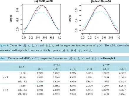
. For ˆgD, [18] proposed an automatic way of choosing the smoothing parameters hN, bn and q. For ˆgN, the

[image:7.595.93.532.390.716.2]

CV approach is used for choosing bandwidth hN.

Figure 1 shows the regression function curve g x

( )

, and the curves of the median MISEs based on 1000 rep-licated estimates of ˆg, ˆgD and ˆgN with η =0.7 under different sample size. From Figure 1, both ˆg and

ˆ_D

g successfully capture the patterns of the true regression curves and have smaller bias than ˆgN. As expected,

ˆ_N

[image:7.595.86.538.599.716.2]

g fails to produce accurate function curve estimates. In addition, it is obvious that the quality of our proposed estimator improve with the increase of sample sizes.

Table 1 compares, for various sample sizes, the results obtained for estimating curve g x

( )

when η =0.7 or η =0.9. The estimated MISEs which were evaluated on a grid of 201 equidistant values of x in

[ ]

0,1 are presented. Our results show that the estimators ˆg and ˆgD outperform ˆgN. It is noteworthy that our proposed

Figure 1. Curves for g xˆ

( )

, gˆ_D

( )

x and gˆ_N

( )

x , and the regression function curve of g x

( )

. The solid, short-dashed, dash-dotted, and long-dashed curves respectively represent g x

( )

, g xˆ

( )

, ˆgD and ˆgN.

Table 1. The estimated MISE ( 2

10−

× ) comparison for estimators g xˆ

( )

, gˆ_D

( )

x and gˆ_N

( )

x in Example 1.

(n N, ) η=0.7 η=0.9

( )

ˆ

g x gˆD( )x gˆN( )x g xˆ( ) gˆD( )x gˆN( )x

3

γ=

(10, 30) 3.7858 5.1262 7.2254 3.8193 3.7822 6.8632

(30, 90) 1.8630 2.2648 4.9030 1.3901 2.7834 5.0495

(60, 180) 1.3056 1.8036 3.9296 0.8524 1.7082 3.7758

5

γ=

(10, 50) 2.2956 3.1562 5.8640 2.0930 3.2097 5.2816

(30, 150) 1.9711 2.1350 4.2684 1.6413 2.0299 4.0137

estimator generally performs better than the estimator proposed by [18] for the resultant MISEs of ˆg are usually smaller. Also, the performance of ˆg improves (i.e. the corresponding MISEs decrease) considerably as the sample sizes increases. For any nonparametric method in measurement error regression problem, the quality of the estimator also depends on the discrepancy of the observed sample. That is, the performance of the esti-mator depends on the variances of measurement error. Here, we compare the results for different values of η. As expected, Table 1 shows that the effect of the variances on the estimator performance is obvious.

Example 2: We considered model (7) with the regression function being

( )

(

)

(

)

_{

_{( )[ ]}2

_}

2 2

, 0,1

, 1 2 1 exp 4 1.4 2 ,

x z

g x z x x z I

∈

 

= −_ − _ − −

and ε being distributed as N

(

0, 0.01

)

. The covariate

(

X Z,

)

T was generated from a bivariate normal dis-tribution N

(

0,Σ

)

with var X

( )

=var Z

( )

=1 and the correlation coefficient between X and Z being 0.6, and

(

)

1 2 2

1

W =ρX+ −ρ v, v~N

( )

0,1 . Then, trim X, W and Z in

[

−2.5, 2.5

]

and scale to

[ ]

0,1 respectively. Results for ρ=0.7 and ρ=0.9 are reported. Simulations were run with different validation and primary da-ta sizes

(

n N,

)

ranging from

(

10, 30

)

to

(

60, 300

)

according to the ratio γ =N n=3 and γ =N n=5, respectively. For each case, 1000 simulated data sets were generated for each sample size of

(

n N,

)

.

Here, we only compared our estimator g x z

( )

, with the naive estimator gN which is the multivariate ker-

nel regression estimator based on the primary dataset

{

(

)

}

1

, , N

i i i _i

Y W Z ₌ , since [18] method cannot be applied to

multivariate cases. Here, we used the Epanechnikov kernel function K x

( )

=0.75 1

(

−x2

)

, x ≤1 for g x z

( )

, and used an product kernel K x x

(

1, 2

)

=K0

( ) ( )

x K1 0 x2 with

( )

2 0

15 9

, 1

8 8

K x = − x + x ≤ for gN. For the

naive estimator gN, bandwidth selection rules were considered by [25]. For our estimator g x z

( )

, , we used

the cross-validation approach to choosing the three parameters hN, hn and q. For this purpose, hn and

(

hN,q

)

are selected separately as follows. Define

(

)

(

)

1 1

ˆ _{; .}

n

N n

Z n h j

j N n

f z h K z Z

nh +

= +

=

∑

−

Here, we adopt the cross-validation (CV) approach to estimate hn by

( )

(

)

{

}

2

1 1

ˆ _{arg min} ˆ _{; ,}

n

N n

j

n j Z j n

h j N

h Z f Z h

n +

−

= +

=

∑

−

where the subscript −j denotes the estimator being constructed without using the jth observation. After ob-taining hˆ_n, we then select

(

h_N,q

)

by

( )

{

( )

(

)

}

2

, 1

1

ˆ _{,ˆ arg min , ;}ˆ_{, , ,}

N

N

i

N i i i n N

h q i

h q Y g W Z h h q

N

−

=

=

∑

− 

where the subscript −i denotes the estimator being constructed without using the ith observation

(

Y W Z_i, _i, _i

)

. We compute MISE at 101 101× grid points of

( )

x z, ranging in

[ ] [ ]

0,1× 0,1 . Table 2 reports the MISE for estimating curves g x z

( )

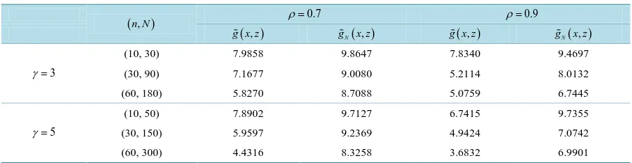
, when ρ =0.7 or ρ =0.9 for various sample sizes. Table 2 shows that our pro-posed estimator substantially outperformed the naive kernel estimator gN. It is obvious that our proposed

esti-mator g has much smaller MISE than gN.

5. Discussion

[image:9.595.85.539.105.222.2]

Table 2. The estimated MISE (×10−2) comparison for the estimators g x z

( )

, and gN

( )

x z, in Example 2.

(n N, ) ρ=0.7 ρ =0.9

( ),

g x z gN( )x z, g x z( ), gN( )x z,

3

γ=

(10, 30) 7.9858 9.8647 7.8340 9.4697

(30, 90) 7.1677 9.0080 5.2114 8.0132

(60, 180) 5.8270 8.7088 5.0759 6.7445

5

γ=

(10, 50) 7.8902 9.7127 6.7415 9.7355

(30, 150) 5.9597 9.2369 4.9424 7.0742

(60, 300) 4.4316 8.3258 3.6832 6.9901

recting the bias arising from the errors-in-variables. It generally preforms better than the approach proposed by [18].

Acknowledgements

This work was supported by NSFC11301245, NSFC11501126 and Natural Science Foundation of Jiangxi Prov-ince of China under grant number 20142BAB211018.

References

[1] Pepe, M.S. and Fleming, T.R. (1991) A General Nonparametric Method for Dealing with Errors in Missing or Surro-gate Covaraite Data. Journal of the American Statistical Association, 86, 108-113.

http://dx.doi.org/10.1080/01621459.1991.10475009

[2] Pepe, M.S. (1992) Inference Using Surrogate Outcome Data and a Validation Sample. Biometrika, 79, 355-365. http://dx.doi.org/10.1093/biomet/79.2.355

[3] Lee, L.F. and Sepanski, J. (1995) Estimation of Linear and Nonlinear Errors-in-Variables Models Using Validation Data. Journal of the American Statistical Association, 90, 130-140.

http://dx.doi.org/10.1080/01621459.1995.10476495

[4] Wang, Q. and Rao, J.N.K. (2002) Empirical Likelihood-Based Inference in Linear Errors-in-Covariables Models with Validation Data. Biometrika, 89, 345-358. http://dx.doi.org/10.1093/biomet/89.2.345

[5] Zhang, Y. (2015) Estimation of Partially Linear Regression for Errors-in-Variables Models with Validation Data.

Springer International Publishing, 322, 733-742. http://dx.doi.org/10.1007/978-3-319-08991-1_76

[6] Xu, W. and Zhu, L. (2015) Nonparametric Check for Partial Linear Errors-in-Covariables Models with Validation Data.

Annals of the Institute of Statistical Mathematics, 67, 793-815. http://dx.doi.org/10.1007/s10463-014-0476-7

[7] Carroll, R.J. and Stefanski, L.A. (1990) Approximate Quasi-Likelihood Estimation in Models with Surrogate Predic-tors. Journal of the American Statistical Association, 85, 652-663. http://dx.doi.org/10.1080/01621459.1990.10474925 [8] Carroll, R.J. and Wand, M.P. (1991) Semiparametric Estimation in Logistic Measurement Error Models. Journal of the

Royal Statistical Society: Series B, 53, 573-585.

[9] Sepanski, J.H. and Lee, L.F. (1995) Semiparametric Estimation of Nonlinear Errors-in-Variables Models with Valida-tion Study.Journal of Nonparametric Statistics, 4, 365-394. http://dx.doi.org/10.1080/10485259508832627

[10] Stute, W., Xue, L. and Zhu, L. (2007) Empirical Likelihood Inference in Nonlinear Errors-in-Covariables Models with Validation Data. Journal of the American Statistical Association, 102, 332-346.

http://dx.doi.org/10.1198/016214506000000816

[11] Cook, J.R. and Stefanski, L.A. (1994) Simulation-Extrapolation Estimation in Parametric Measurement Error Models.

Journal of the American Statistical Association, 89, 1314-1328. http://dx.doi.org/10.1080/01621459.1994.10476871 [12] Carroll, R.J., Gail, M.H. and Lubin, J.H. (1993) Case-Control Studied with Errors in Covariables. Journal of the

American Statistical Association, 88, 185-199.

[13] Lü, Y.-Z., Zhang, R.-Q. and Huang, Z.-S. (2013) Estimation of Semi-Varying Coefficient Model with Surrogate Data and Validation Sampling. Acta Mathematicae Applicatae Sinica, English Series, 29, 645-660.

http://dx.doi.org/10.1007/s10255-013-0241-3

[15] Yu, S.H. and Wang, D.H. (2014) Empirical Likelihood for First-Order Autoregressive Error-in-Variable of Models with Validation Data. Communications in Statistics Theory Methods, 43, 1800-1823.

http://dx.doi.org/10.1080/03610926.2012.679763

[16] Stefanski, L.A. and Buzas, J.S. (1995) Instrumental Variable Estimation in Binary Regression Measurement Error Models. Journal of the American Statistical Association, 90, 541-550.

http://dx.doi.org/10.1080/01621459.1995.10476546

[17] Wang, Q. (2006) Nonparametric Regression Function Estimation with Surrogate Data and Validation sampling. Jour-nal of Multivariate AJour-nalysis, 97, 1142-1161. http://dx.doi.org/10.1016/j.jmva.2005.05.008

[18] Du, L., Zou, C. and Wang, Z. (2011) Nonparametric Regression Function Estimation for Error-in-Variable Models with Validation Data. Statistica Sinica, 21, 1093-1113. http://dx.doi.org/10.5705/ss.2009.047

[19] Carroll, R.J., Ruppert, D., Stefanski, L.A. and Crainiceanu, C.M. (2006) Measurement Error in Nonlinear Models. Second Edition, Chapman and Hall CRC Press, Boca Raton. http://dx.doi.org/10.1201/9781420010138

[20] Hall, P. and Horowitz, J.L. (2005) Nonparametric Methods for Inference in the Presence of Instrumental Variables.

Annals of Statistics, 33, 2904-2929. http://dx.doi.org/10.1214/009053605000000714

[21] Darolles, S., Florens, J.P. and Renault, E. (2006) Nonparametric Instrumental Regression. Working Paper, GREMAQ, University of Social Science, Toulouse.

[22] Newey, W.K. and Powell, J.L. (2003) Instrumental Variable Estimation of Nonparametric Models. Econometrica, 71, 1565-1578. http://dx.doi.org/10.1111/1468-0262.00459

[23] Blundell, R., Chen, X. and Kristensen, D. (2007) Semi-Nonparametric IV Estimation of Shape-Invariant Engel Curves.

Econometrica, 75, 1613-1669. http://dx.doi.org/10.1111/j.1468-0262.2007.00808.x

[24] Newey, W.K. (1997) Convergence Rates and Asymptotic Normality for Series Estimators. Journal of Econometrics,

79, 147-168. http://dx.doi.org/10.1016/S0304-4076(97)00011-0

[25] Schimek, M.G. (2012) Variance Estimation and Bandwidth Selection for Kernel Regression. John Wiley & Sons, Inc., New York, 71-107.

Appendix

Proof of Theorem 1

Let T*:L2

( )

χ →L2

( )

χ denotes the adjoint operator of T. Under assumption A1(ii), the self-adjoint operators

of TT* and T T* have the same eigenvalue sequence

{ }

µk2 with

2 2 1 1 2

µ = ≥µ ≥_ Moreover, we assume that the corresponding eigenfunctions of the operators TT* and T T* are also orthonormal basis

{

φ_k,k=1, 2,

}

, and for all k≥1

* * 2 * 2

, ; , .

k k k k k k k k k k k k

Tφ =µ φ Tφ =µ φ T Tφ =µ φ TTφ =µ φ Define

( )

( )

( )

( )

1 1

, and .

q q

n k k N k k

k k

g x gφ x m w mφ w

= =

=

∑

=

∑

Let Tn be the operator whose kernel is

(

)

( ) ( )

1 1

, ,

q q

n kl k l

k l

t x w d φ x φ w

= =

=

∑∑

then T gn n =mN. By the definition of ns, we have gn∈ns.

Lemma 1. Under conditions A1 and A3(i) and the sieve space ns, we have

1) T g

{

−g_n

}

≤const.×µ_q× g−g_n ; 2) τn≤1µq.

Lemma 2. Under conditions A1,A3(ii) and A4, we have

{

_ˆ

}

(

1 2 1 2

)

sup .

ns

r d

n P

T T O q q n

ϕ ϕ

− −

∈ − = +

By some modifications of the proof of Theorem 2 in [23] and applying the Theorem 7 in [24], the proofs of Lemma 1 and Lemma 2 are straightforward and are omitted.

Proof of Theorem 1. By the triangle inequality, we have

ˆ ˆ _{n n} .

g−g ≤ g−g + g −g

By the definition of ns and condition A3(i), we have

(

s d

)

.

n

g −g =O q− (12)

see e.g. [26] for Fourier series.

Next, by the definition of τn and the triangle inequality, we have

(

)

ˆ _{n n} ˆ _n .

g−g ≤τ T g−g

We now analyze the term T g

(

ˆ−g_n

)

. By the triangle inequality, we have

(

)

(

)

(

)

(

)

(

)

ˆ ˆ

ˆ ˆ ˆ ˆ ˆ

ˆ _ˆ ˆ _{ˆ ˆ ˆ .}

n n n n

n n n

T g g T T g T g m m m T g g

T T g T g m m m T g g

− = − + − + − + −

≤ − + − + − + −

By conditions A2, A4 and central limit theorem, we can show that mˆ−Emˆ =O_P_

(

q N

)

1 2_. From condi-tion A3(ii), we have ˆ

(

r d

)

Em−m =O q− . Hence, _ˆ

(

r d 1 2 1 2

)

P

m−m =O q− +q N− . In addition, by the

defini-tion of ˆg and the triangle inequality, we have

(

)

(

)

ˆ _{ˆ ˆ} ˆ _ˆ ˆ _{ˆ .}

n n n n n n

T g−m ≤ T g −m ≤ T −T g + T g −g + m m−

These and Lemma 2 imply

(

)

(

(

)

)

{

1 2 1 2 1 2 1 2

}

ˆ n n P r d n .

This and Lemma 1 imply

(

1 2 1 2 1 2 1 2

)

ˆ _{n n P} r d .

g−g ≤ g−g + ×τ O q− +q N− +q n− (13) The theorem follows immediately from (12)-(13).

Proof of Theorem 2

Lemma 3. For each z∈

[ ]

0,1p, define

( )

( )

( )

( )

1 1

, and .

q q

zn zk k zN zk k

k k

g x g φ x m w m φ w

= =

=

∑

=

∑

Let Tzn be the operator whose kernel is

(

)

( ) ( )

1 1

, ,

q q

zn zkl k l

k l

t x w d φ x φ w

= =

=

∑∑

then T gzn zn =mzN. By the definition of ns, we have gzn∈ns.

Proof of Theorem 2. For each z∈

[ ]

0,1 p, by the triangle inequality, we have

( )

,

( )

, _{zn zn zn z}

(

_zn

)

_zn ,

g x z −g x z ≤ g−g + g −g ≤τ × T g−g + g −g By assumption B3(i), it is easy to show that

(

s d

)

zn

g −g =O q− . Similar to the proof of Theorem 1, we have

(

)

(

ˆ

)

ˆ _{ˆ ˆ}

(

)

_.

z zn z zn zn z zn

T g−g ≤ T −T g + T g−m + m m− + T g−g

According to assumptions B2, B3(ii), B4, and B5(i), we can show that ˆ ˆ

(

1 2 r(2r p)

)

P

m−Em =O q N− + ,

( )

(

1 2 2

)

ˆ r r p r d

Em m− =O q N− + +q− . In addition, by some modifications of the proof of Lemma 2, under

as-sumptions B1, B3(ii), B4, B5(i) and B6, we have

{

_ˆ

}

(

1 2 (2 )

)

sup .

ns

r r p r d

zn P

T T O q q n

ϕ ϕ

− +

−

∈ − = +

For the term Tz

(

gzn−g

)

, under assumptions B1, B3(i) and the sieve space ns, we have

(

)

const.

zn Tz gzn g g gzn

τ × − ≤ × −