Future meat consumption: potential greenhouse gas emissions from meat production in Malaysia

Munich Personal RePEc Archive

Future meat consumption: potential

greenhouse gas emissions from meat

production in Malaysia

Tey, (John) Yeong-Sheng

15 January 2009

Online at

https://mpra.ub.uni-muenchen.de/14534/

FUTURE MEAT CONSUMPTION: POTENTIAL GREENHOUSE GAS EMISSIONS FROM MEAT PRODUCTION IN MALAYSIA

by

Tey (John) Yeong-Sheng1

ABSTRACT

This study shows that there is mounting meat consumption which is to be met by higher meat

production. As the result, higher gas emission of CO2 is expected from increasing meat

production. This is led by poultry and beef production which is likely to produce most of the greenhouse gas emissions from meat production in Malaysia. It is crucial to incorporate environmental consideration into livestock policy in National Agricultural Policy 4 and Tenth Malaysian Plan.

Keywords: Meat, consumption, production, gas emission.

JEL code: Q11, Q50

1.0 INTRODUCTION

The ultimate intention in Malaysian agri-food policies is to increase agri-food production, for self-sufficiency and trade. However, the policies tend to hold the grip on the economic impact of the industry rather than the profound environmental impacts caused by agricultural activities. One of the myriad impacts is greenhouse gas emissions from meat production. A

recent study by Steinfeld et al. (2006) found that the production of meat contributes between 4.6

and 7.1 billion tonnes of greenhouse gases each year, which represents between 15% and 24% of total current greenhouse gas production.

At aggregate level, the domestic meat consumption pattern is like those described by

Keyzer et al. (2005) as per capita total meat consumption has increased over the years, at a very

high rate. Relatively, beef consumption has increased faster than other major meat products (poultry, pork, and mutton) at the fast track of economic growth after 1997/98. This leads to the question of what would be the future meat consumption at disaggregate level.

The consumer-driven meat sector is well spelt in the National Agricultural Policy 3. While the demand is mounting, beef and mutton are still self-insufficient at large in domestic market. The unfulfilled demand is expected to see a boost in beef and mutton production.

1

Corresponding author

Email: tyeong.sheng@gmail.com

Coupled with all-time high poultry and pork production, it is essential to investigate possible greenhouse emission from meat production in Malaysia. Hence, this study intends to (1) forecast for future meat consumption and production, and (2) generate potential future greenhouse gas emissions from meat production in Malaysia.

2.0 DATA AND ESTIMATION PROCEDURES

Time-series data of beef, pork, mutton, and pork consumption and self-sufficiency level are obtained from various issues of Agriculture Statistical Handbook (1960-2008). Several series of data namely 1960-2008, 1970-2008, 1980-2008, and 1990-2008 are analyzed via simple linear regressions from managerial economics perspective. This is to choose the best series which produce the least residuals. The simple linear regression can be expressed as:

TT

Qi) 0i 1i

log(   

where Q is consumption (quantity) of ith meat product and TT is time trend in the data series.

The forecast can then be done by plugging the continuous time trend up to 2020 into the estimated linear regression. However, the projection is not meant to be deterministic. Stochastically, the projection is shift upward and downward based on the average percentage of residuals in the observations.

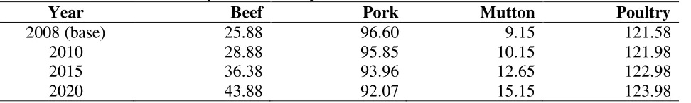
In order to obtain forecast of meat production, information of future self-sufficiency level for the major meat products are needed. Table 1 presents the calculated meat self-sufficiency level in Malaysia, which was estimated by adding average annual growth of 1.5, -0.38, 0.5, and 0.2 to the base (2008) of self-sufficiency level in beef, pork, mutton, and poultry respectively. It is noteworthy that self-sufficiency level in beef, mutton, and poultry are aligned with the target in Ninth Malaysian Plan, whereas pork performs negatively.

Table 1: Meat self-sufficiency level in Malaysia

Year Beef Pork Mutton Poultry

2008 (base) 25.88 96.60 9.15 121.58

2010 28.88 95.85 10.15 121.98

2015 36.38 93.96 12.65 122.98

2020 43.88 92.07 15.15 123.98

Forecast for meat production is then yielded by multiplying the forecasted meat consumption with the forecasted self-sufficiency level. Then, the forecasted meat production is

transformed into greenhouse CO2 quantity by using the estimates as shown in Table 2.

Table 2: Greenhousegas impact of 1kg of a given meat product

Year Beef Pork Mutton Poultry

CO2 equivalent (kg) 36.4i 3.8ii 13.8iii 1.1 iii

Notes: i Koneswaran and Nierenberg (2008); ii Pimentel (1997), and iii Eshel and Martin (2006)

5.15 5.2 5.25 5.3 5.35

0 5 10 15 20

Time trend P o rk c o n su m p ti o n 5.4 5.5 5.6 5.7 5.8 5.9 6 6.1

0 5 10 15 20

Time trend P o u lt ry c o n su m p ti o n

3.0 RESULTS

The best model specification was chosen based on the lowest residuals criteria in the observations. Given the lower residual values in the data series of 1990-2008, the data series was consistently the better one to use in the analysis of the major meat products in Malaysia. Graphically, they are illustrated in Figure 1. The straight lines represent predicted consumption values while having actual consumption values tabulated around them. The gap between the lines and actual consumption values is known as residuals. The average of residual is about 5 percent annually for beef, mutton, and poultry consumption. In the case of pork consumption, there are highs and lows mainly due to consumption shock in view of disease outbreak in the industry. Though so, the annual average residual is about 10 percent.

Figure 1: Plot of fit line

4.6 4.7 4.8 4.9 5 5.1 5.2 5.3

0 5 10 15 20

Time trend B ee f co n su m p ti o n

(a) Beef consumption (b) Pork consumption

3.8 3.9 4 4.1 4.2 4.3 4.4

0 5 10 15 20

Time trend M u tt o n c o n su m p ti o n

(c) Mutton consumption (d) Poultry consumption

Table 3: Linear regression parameters

Beef Pork Mutton Poultry

Coefficients Coefficients Coefficients Coefficients

(Std. error) (Std. error) (Std. error) (Std. error)

Intercept 3.93 5.19 3.88 5.53

(0.03)*** (0.02)*** (0.02)*** (0.02)***

Time trend 0.03 0.01 0.02 0.03

(0.00)*** (0.00)*** (0.00)*** (0.00)***

Note: *** Statistically significant at 1% level of significance.

By plugging continuous time trend values into the parameters, an initial projection for the major products was obtained. In order to make it to be stochastic, projected beef, mutton, and poultry consumption was adjusted by 5 percent (as indicated by the average residual) and projected pork consumption was adjusted by 10 percent respectively. The stochastic projection of meat consumption is depicted in Table 4. The range of the projected consumption values is to indicate that the future consumption will fall within the range, which tolerates reduction and increase in the range. Meat consumption is projected to increase in future. Most strikingly is the rising beef consumption that overtakes pork consumption.

Table 4: Stochastic projection of meat consumption

Year Beef (M. Ton.) Pork (M. Ton.) Mutton (M. Ton.) Poultry (‘000 M. Ton.)

5% lower 5% upper 10% lower 10% upper 5% lower 5% upper 5% lower 5% upper

2010 154,348 170,596 188,303 230,149 22,470 24,836 1,146,820 1,267,538 2015 206,054 227,744 201,744 246,575 29,463 32,565 1,551,582 1,714,906 2020 275,079 304,035 216,143 264,175 38,632 42,698 2,099,201 2,320,169

By multiplying the projected meat consumption with self-sufficiency level, Table 5 presents the estimated stochastic projection of local meat production. As spelt out in the self-sufficiency level in earlier session, beef production is expected to grow faster than other meat products. It is interesting to learn that poultry and pork production tends to increase at marginal rate.

Table 5: Stochastic projection of local meat production

Year Beef (M. Ton.) Pork (M. Ton.) Mutton (M. Ton.) Poultry (‘000 M. Ton.)

5% lower 5% upper 10% lower 10% upper 5% lower 5% upper 5% lower 5% upper

2010 44,576 49,268 180,489 220,597 2,281 2,521 1,398,891 1,546,143

2015 74,962 82,853 189,558 231,682 3,726 4,118 1,908,135 2,108,991

2020 120,704 133,410 199,003 243,226 5,853 6,469 2,602,589 2,876,545

Table 6 illustrates the increasing gas emission from local meat production. Obviously, the

increasing meat production has direct impact on environment, in term of gas emission - CO2.

Table 6: Stochastic projection of gas emission from local meat production

Year

Beef (M. Ton.) Pork (M. Ton.) Mutton (M. Ton.) Poultry (‘000 M. Ton.)

Low variant High variant Low variant High variant Low variant High variant Low variant High variant

2010 1,622,566 1,793,355 685,858 838,269 31,478 34,790 1,538,780 1,700,757

2015 2,728,617 3,015,849 720,320 880,392 51,419 56,828 2,098,949 2,319,890

2020 4,393,626 4,856,124 756,211 924,259 80,771 89,272 2,862,848 3,164,200

4.0 CONCLUSIONS

This study follows the flow of a consumer-driven agri-food market to (1) forecast for future meat consumption and production, and (2) generate potential future greenhouse gas emissions from meat production in Malaysia. The empirical results show that there is mounting meat

consumption which is to be met by higher meat production. As the result, gas emission of CO2

are expected to increase from meat production, with other things remain unchanged. Having such indications, it is crucial to incorporate environmental consideration into livestock policy in National Agricultural Policy 4 and Tenth Malaysian Plan.

REFERENCES

Agriculture Statistical Handbook (various issues), Ministry of Agriculture and Agro based Industries.

Eshel, G., Martin, P. (2006). Diet, Energy and Global Warming, Earth Interactions, 10, 1–17.

Keyzer, M.A., Merbis, M.D., Pavel, I.F.P.W., van Wesenbeeck, C.F.A. (2005). Diet Shifts

Towards Meat and The Effects on Cereal Use: Can We Feed The Animals in 2030? Ecological

Economics, 55 (2), 187–202.

Koneswaran G, Nierenberg D. (2008). Global Farm Animal Production and Global Warming:

Impacting and Mitigating Climate Change, Environ Health Perspect, 116: 578–582.

Pimentel, D. (1997). Livestock Production: Energy Inputs and The Environment. In: Scott, SL, Zhao, X (Eds.), Canadian Society of Animal Science, Proceedings, Vol. 47. Canadian Society of Animal Science, Montreal, Canada, pp. 17–26.