LPM Density Functions for the Computation of the SD Efficient Set

(1)

http://dx.doi.org/10.4236/jmf.2016.61012

How to cite this paper: Viole, F. and Nawrocki, D. (2016) LPM Density Functions for the Computation of the SD Efficient Set. Journal of Mathematical Finance, 6, 105-126. http://dx.doi.org/10.4236/jmf.2016.61012

LPM Density Functions for the Computation

of the SD Efficient Set

Fred Viole

1

, David Nawrocki

2

1_{OVVO Financial Systems, Holmdel, USA}

2_{Villanova University, Villanova School of Business, Villanova, USA}

Received 22 October 2015; accepted 23 February 2016; published 26 February 2016

This work is licensed under the Creative Commons Attribution International License (CC BY).

http://creativecommons.org/licenses/by/4.0/

Abstract

The equivalence between partial moments and stochastic dominance dates back to Bawa [1] and Fishburn [2]. We present a test for first, second, and third degree stochastic dominance between two variables using Lower Partial Moments. The results uphold Hadar and Russell’s [3] original conclusions about the odd moments of preferred prospects. We recall Nawrocki’s [4] research comparing Mean/Variance portfolios against the continuum of risk-averse investors using Lower Partial Moments. The excess skewness of the LPM portfolios clearly demonstrates the preference of positive skewness for risk-averse investors. Finally, we provide an algorithm for efficiently de-termining stochastic dominance efficient sets among large numbers of variables.

Keywords

Stochastic Dominance Algorithm, Lower Partial Moments, Expected Utility Theory, Prospect Theory, Upper Partial Moments

1. Introduction

(2)

106

stochastic dominance can be run on thousands of securities and portfolio optimization algorithms are limited to about 150 securities due to singularity errors.1 In this paper, we propose using a stochastic dominance algorithm using lower partial moments for step (1) and then using mean-semivariance or UPM/LPM algorithm for step (2).2

The use of semivariance or lower partial moment analysis to approximate stochastic dominance has already been suggested. Bey [5] proposes a mean-semivariance algorithm to approximate the second degree stochastic dominance efficient portfolio sets. More importantly, Bawa [1] and Fishburn [2] provide proofs for the equiva-lence of LPM degrees greater than one to second degree stochastic dominance and for LPM degrees greater than two to third degree stochastic dominance.3

Since stochastic dominance is an analysis of cumulative distribution functions; only below target deviations are considered over the interval [−∞, target] with the target encompassing all values of X. This “for all X” target condition is directly responsible for the generalization to all possible risk averse utility assumptions.

This paper proposes an integration of stochastic dominance analysis and lower partial moment analysis by de-fining a stochastic dominance (SD) test via the Lower Partial Moments (LPM) of the investment’s probability distribution. From this SD-LPM test, we can quickly and efficiently determine the SD efficient set and generate optimal portfolios from that reduced universe of securities for any objective function (Mean/Variance, UPM/ LPM, etc.). Equation (1) represents the LPM of an investment,

(

)

{

(

)

}

1

, , max , 0

T _n

t t

LPM n h X h X

T =

=

∑

− (1)

where X_t is the observation of variable X at time t; h is the target from which to compute the lower deviation; and n is the loss aversion weight assigned to the lower deviation. The next section explains the equivalence be-tween LPM and SD for First Degree Stochastic Dominance (FSD), Second Degree Stochastic Dominance (SSD) and Third Degree Stochastic Dominance (TSD). In Section 3 we discuss the methodology of the SD routines and the SD efficient set algorithm. The appendices contain R code, commentary on the R code and working examples. In these examples we note the effects of SD on the odd moments of the distributions, consistent with Hadar and Russell [1969] original conclusions.

2. Historical Partial Moment Equivalence & Tests

Bawa [1] provides a proof that the LPM measure is mathematically related to stochastic dominance for risk to-lerance values (n) of 0, 1, and 2. Fishburn [2] demonstrates the equivalence of the LPM measure to stochastic dominance for all values of n > 0. He provides the general case via:

( )

h

(

)

nd

( )

. n

F h =

∫

_−∞ h−X F X (2)

Fishburn [2] also shows that the n value includes all types of investor behavior. Furthermore, Porter [10] illu-strates that except for cases of identical means and semivariances, if X dominates Y by second degree stochastic dominance then X dominates Y by the mean-target semivariance model. Building from the general case, let F_X denote the cumulative distribution function of variable X such that:

(

0, ,

)

_X

( )

LPM h X =F h (3)

(

1, ,

)

h

(

) ( )

d

LPM h X =

∫

_−∞ h−X F X (4)

(

)

(

)

2

( )

2, , h d .

LPM h X =

∫

_−∞ h−X F X (5)

Therefore, Equation (3) will be the statistic used for FSD testing, Equation (4) will be the statistic used for SSD testing, and Equation (5) will be the statistic used for TSD testing. We note that Equation (3) is a probabil-ity whereby the target deviation is taken to the 0th degree. The LPM degree 0 is simply the empirical cumulative

1_{Private correspondence with Harry Markowitz on the limits to the critical line algorithm. Markowitz}_[6]_{also recommends geometric mean-}

semivariance as the appropriate MPT approach.

2_{See Nawrocki}_[7]_{for a review of lower partial moment (LPM) risk measures.}

3_{Although Tehranian}_[8]_{and Helms, Jean, and Tehranian}_[9]_{suggested stochastic dominance degrees greater than three and the fact is that}

(3)

107

distribution function (CDF) of the distribution. When considering how far a deviation is from its target, increas-ing the degree per Equation (4) will give a linear weightincreas-ing. This is the area of the distribution to the left of the target, h. Finally, if an investor is more sensitive to below target observations, increasing the degree further will compensate this behavior. The LPM Degree 2 used in Equation (5) is equivalent to the semivariance statistic. These equations must be used from every target in the return distribution to generalize for all risk-averse inves-tor types.

In a bid to infer SD from aggregate statistics (and skip the every target “for all h” inconvenience), others have suggested various CDF tests to approximate SD results. For example, Klecan et al. [11] proposes a difference in CDFs, per the Kolmogorov-Smirnoff (KS) test, further bolstered by Monte Carlo simulation for robustness. However, the KS test used does not prove FSD or SSD. The test statistic, D=maxFX

( )

h −FY

( )

h  is

defi-cient because it does not satisfy the “for all h” previously alluded to. FSD is a very stringent qualification, whe-reby one observation in which F_X >F_Y nullifies X FSD Y. What you have is a statistically significant differ-ence in CDFs, which unfortunately does not tell us anything about stochastic dominance. Of course Klecan et al.

[11] realize this and alter their hypothesis to test for a variable that is not stochastically maximal, i.e. weak sto-chastic dominance holds for some pair of prospects within their observed set.

“The set A is first-degree [resp., second-degree] maximal if no prospect in A is weakly stochastically dom-inated by another prospect in A. First-degree dominance implies second-degree dominance, and second- degree maximality implies first degree maximality.” Klecan et al. [11].

Developing an efficient routine to determine SD was originally hampered by computing power coupled with arcane techniques. Computing power has increased dramatically since the 1970s, thus enabling portfolio sizes unattainable back then. Furthermore, the use of partial moments are a computationally efficient method of de-termining CDFs flexible enough for the entire distribution and extending themselves to area analysis required for the higher SD degrees.

“Finally, in order to conduct tests of SSD efficiency, all the calculations required for the FSD test must be made regardless of whether one is interested in FSD results; for TSD experiments, all the calculations re-quired for FSD and SSD tests must be made.” Porter, Wart and Ferguson [12].

The use of LPMs in the SD test eliminates the calculation redundancy Porter et al. [12] noted above. In fact, TSD takes less time to run than FSD per our routines, the explanation of which follows.

2.1. SD Routines

A complete presentation of the R code and commentary on the modules is presented in the Appendix A and Appendix C of this paper. Here, we are providing a general overview of how each SD routine performs its task on individual securities or aggregate portfolios.

2.1.1. FSD

To determine FSD between two variables we combine the observations into a single vector. Next we rank the observations in ascending order. This is the target vector. Using the combined sorted observations we compare CDFs from each target using Equation (3).

If the LPM

(

0, target ,_i X

)

<LPM

(

0, target ,_i Y

)

then we store the instance with a binary indicator into an output vector. If at any target the relationship fails, the routine is stopped and the result of “No FSD Exists” is returned. This has the benefit of avoiding all of the observations as soon as a violation is detected. Otherwise we continue through the rest of the target vector until all observations are exhausted, thus affirming “XFSD Y” exis-tence.

In an added bid of efficiency we incorporate an additional output vector for Y such that it can be checked si-multaneously for “Y FSD X”.

2.1.2. SSD

(4)

If the LPM

(

1, target ,_i X

)

<LPM

(

1, target ,_i Y

)

then we store the instance with a binary indicator into an output vector. All of the benefits from the FSD routine are preserved.

2.1.3. TSD

Again, using the identical combined sorted observation vector (yet another efficiency since it does not have to be generated for each degree tested) the two variables of interest are compared with their squared areas below a target, or simply their semivariance. Equation (5) represents this consideration.

If the LPM

(

2, target ,_i X

)

<LPM

(

2, target ,_i Y

)

then we store the instance with a binary indicator into an output vector for that specific target. All of the benefits from the FSD and SSD routines are preserved.

2.2. SD Efficient Set

We incorporate these SD routines into a “SD Efficient Set” algorithm. The specific R code is also provided in the Appendix C. A full discussion of the algorithm is in Appendix A using a data frame (a list of vectors of equal lengths in R) of security or portfolio returns, we are able to generate the SD efficient set for the desired degree and return a reduced data frame. A visualization of the problem is presented by borrowing a reference to Braid Theory, which is an abstract geometric theory studying the everyday braid concept.

Our first step is to rank the securities or portfolios in ascending order by their LPM from the maximum ob-servation across all variables. Using the terms “Base” and “Challenger” from Porter et al. [12], our first ranked variable is our “Base”. The next ranked variable is the “Challenger”. We test whether “Base” SD “Challenger”. If “Base” SD “Challenger”, then “Challenger” is placed in a “Dominated Set” which is an output vector. If “Base” does not SD “Challenger” then “Challenger” is added to the “Base” vector. The next “Challenger” must be tested against all members of the current “Base” vector. If it fails but one, it is immediately placed in the “Dominated Set” and the next “Challenger” is selected. When all “Challengers” are exhausted, the final SD Ef-ficient Set is simply the original data frame less the “Dominated Set”.

2.3. SD Algorithm Empirical Results

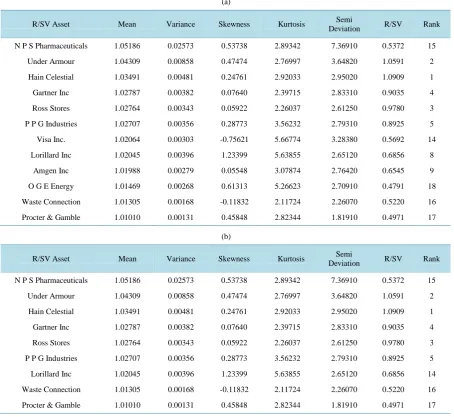
The resulting SD Efficient data frame can then be easily implemented (within the same command line) into an optimization routine. We verify the output from our method versus the DOMIN1 routine originally presented in Porter et al. [12] with the third degree SD correction suggested by Bey, Burgess, and Kearns [13]. We obtained a monthly total return dataset of 67 stocks from the CRSP dataset for the period 2010 to 2014. Summary statis-tics are provided in Appendix B. We then used the DOMIN1 routine and our R code routine to generate the FSD, SSD, and TSD efficient sets. Indeed the same securities are selected from a 67 security universe. The results for the SSD and TSD analysis are presented in Table 1.

One potential question is whether a simple reward to semivariability (R/SV) ratio ranking would be equiva-lent to the LPM SD algorithm. Table 1 results indicate the answer is no. We ranked all 67 companies by R/SV ratio with the last column in Table 1 indicating the company’s rank among the 67 companies. For the SSD re-sults, there are 12 undominated companies and only 7 companies are ranked in the top 12 of the R/SV rankings (5 companies are ranked out of the top 12). For the TSD results, there are 9 undominated companies and only 6 companies are ranked in the top 9 of the R/SV rankings (3 are ranked out of the top 12).

3. Discussion

While stochastic dominance implies mean/Semivariance or LPM dominance, LPM dominance does not imply stochastic dominance because of the nature of aggregate statistics versus individual observations. This is ana-logous to the common phrase: “While dependence implies correlation, correlation does not imply dependence.” The stringent criterion of stochastic dominance defies implication from aggregate distributional statistics.

Given LPM’s ability to consider multiple investor preferences, from a practical standpoint, it seems the best candidate to proxy stochastic dominance. We demonstrated how skewness is evident under SSD and TSD. This is not surprising given Nawrocki’s [4] analysis of LPM portfolios versus their M/V counterparts, whereby excess positive skewness was an artifact of all risk-averse investors.

(5)

[image:5.595.86.541.125.542.2]

109

Table 1. Second and third degree undominated assets from 67 stocks, monthly data from January 2010 to December 2014 using DOMIN1 and our R code. The mean return is a monthly return relative and the Semi Deviation is a monthly percent

change. (a) Second degree (SSD) undominated assets; (b) Third degree (TSD) undominated assets.

(a)

R/SV Asset Mean Variance Skewness Kurtosis Semi

Deviation R/SV Rank

N P S Pharmaceuticals 1.05186 0.02573 0.53738 2.89342 7.36910 0.5372 15

Under Armour 1.04309 0.00858 0.47474 2.76997 3.64820 1.0591 2

Hain Celestial 1.03491 0.00481 0.24761 2.92033 2.95020 1.0909 1

Gartner Inc 1.02787 0.00382 0.07640 2.39715 2.83310 0.9035 4

Ross Stores 1.02764 0.00343 0.05922 2.26037 2.61250 0.9780 3

P P G Industries 1.02707 0.00356 0.28773 3.56232 2.79310 0.8925 5

Visa Inc. 1.02064 0.00303 -0.75621 5.66774 3.28380 0.5692 14

Lorillard Inc 1.02045 0.00396 1.23399 5.63855 2.65120 0.6856 8

Amgen Inc 1.01988 0.00279 0.05548 3.07874 2.76420 0.6545 9

O G E Energy 1.01469 0.00268 0.61313 5.26623 2.70910 0.4791 18

Waste Connection 1.01305 0.00168 -0.11832 2.11724 2.26070 0.5220 16

Procter & Gamble 1.01010 0.00131 0.45848 2.82344 1.81910 0.4971 17

(b)

R/SV Asset Mean Variance Skewness Kurtosis Semi

Deviation R/SV Rank

N P S Pharmaceuticals 1.05186 0.02573 0.53738 2.89342 7.36910 0.5372 15

Under Armour 1.04309 0.00858 0.47474 2.76997 3.64820 1.0591 2

Hain Celestial 1.03491 0.00481 0.24761 2.92033 2.95020 1.0909 1

Gartner Inc 1.02787 0.00382 0.07640 2.39715 2.83310 0.9035 4

Ross Stores 1.02764 0.00343 0.05922 2.26037 2.61250 0.9780 3

P P G Industries 1.02707 0.00356 0.28773 3.56232 2.79310 0.8925 5

Lorillard Inc 1.02045 0.00396 1.23399 5.63855 2.65120 0.6856 14

Waste Connection 1.01305 0.00168 -0.11832 2.11724 2.26070 0.5220 16

Procter & Gamble 1.01010 0.00131 0.45848 2.82344 1.81910 0.4971 17

The Bey-Kearns-Burgess [13] TSD Correction in DOMIN1 Has Been Activated. The Number of Check Points = 6; ITEST = 1; JTEST = 3.

variances. This is verified with a 67 security universe example providing identical outputs for SSD and TSD. One potential weakness of any empirical risk analysis approach is estimation error. Both SD and LPM are nonparametric and do not require knowledge of the underlying probability function. In simulation tests that we have conducted, the LPM measures are less sensitive to estimation error than either the mean or variance no matter which distribution is assumed.

(6)

functions by Levy and Levy [16] [17], Post and Levy [18], Baltussen, Post and van Vliet [19], andPost, van Vliet and Levy [20].

In order to generalize further, one would have to expand the analysis into an Upper Partial Moment/Lower Partial Moment (UPM/LPM) framework, capable of incorporating the often observed four-fold pattern of risk behavior identified in prospect theory and expected utility theory such as the UPM/LPM optimization model described by Viole and Nawrocki [21][22] and Cumova and Nawrocki [23].

4. Conclusions

The close relationship between lower partial moments and stochastic dominance has been known since Porter

[10], Bawa [1], Fishburn [2], and Bey [5]. This paper uses the known cumulative density function properties and utility function properties of lower partial moments to generate stochastic dominant efficient sets. We hope that this paper demonstrates how powerful LPM analysis potentially is for statistical/financial analysis (and by ex-tension UPM/LPM analysis). An efficient algorithm to generate SD efficient sets is proposed and tested along-side with the Porter et al. [12]. DOMIN1 algorithm which includes the third degree SD correction is suggested by Bey et al. [13]. Both algorithms provided the same efficient sets for SSD and TSD for a sample 67 security universe. A description of the LPM SD algorithm is provided in Appendix A and the R-code for the algorithm is included in Appendix C.

Future research should extend the analysis to the use of UPM/LPM models which are superior to SD and LPM models for incorporating the full range of utility functions available with expected utility theory and pros-pect theory.

References

[1] Bawa, V.S. (1975) Optimal Rules for Ordering Uncertain Prospects. Journal of Financial Economics, 2, 95-121. [2] Fishburn, P. (1977) Mean-Risk Analysis with Risk Associated with Below-Target Returns. American Economic

Re-view, 67, 116-126.

[3] Hadar, J. and Russel, W.R. (1969) Rules for Ordering Uncertain Prospects. The American Economic Review, 59, 25- 34.

[4] Nawrocki, D. (1992) The Characteristics of Portfolios Selected by N-Degree Lower Partial Moment. International Re-view of Financial Analysis, 1, 195-209. http://dx.doi.org/10.1016/1057-5219(92)90004-N

[5] Bey, R.P. (1979) Estimating the Optimal Stochastic Dominance Efficient Set with a Mean-Semivariance Algorithm.

Journal of Financial and Quantitative Analysis, 14, 1059-1070.

[6] Markowitz, H.M. (2010) Portfolio Theory: As I Still See It. Annual Review Financial Economics, 2, 1-23.

http://dx.doi.org/10.1146/annurev-financial-011110-134602

[7] Nawrocki, D. (1999) A Brief History of Downside Risk Measures. The Journal of Investing, 8, 9-25.

http://dx.doi.org/10.3905/joi.1999.319365

[8] Tehranian, H. (1980) Empirical Studies in Portfolio Performance Using Higher Degrees of Stochastic Dominance. The Journal of Finance, 35, 159-171. http://dx.doi.org/10.1111/j.1540-6261.1980.tb03478.x

[9] Helms, B.P., Jean, W.H. and Tehranian, H. (1986) An Algorithm for NTH Degree Stochastic Dominance. Applied Stochastic Models and Data Analysis, 2, 71-81. http://dx.doi.org/10.1002/asm.3150020107

[10] Porter, R.B. (1974) Semivariance and Stochastic Dominance: A Comparison. The American Economic Review, 64, 200-204.

[11] Klecan, L., McFadden, R. and McFadden, D. (1991) A Robust Test for Stochastic Dominance. Working Paper, De-partment of Economics, MIT, Cambridge.

[12] Porter, R.B., Wart, J.R. and Ferguson, D.L. (1973) Efficient Algorithms for Conducting Stochastic Dominance Tests on Large Numbers of Portfolios. Journal of Financial and Quantitative Analysis, 8, 71-81.

http://dx.doi.org/10.2307/2329749

[13] Bey, R.P., Burgess, R.C. and Kearns, R.B. (1984) Moving Stochastic Dominance: An Alternative Method for Testing Market Efficiency. Journal of Financial Research, 7, 185-196. http://dx.doi.org/10.1111/j.1475-6803.1984.tb00369.x

[14] Whitmore, G.A. (1970) Third-Degree Stochastic Dominance. The American Economic Review, 60, 457-459.

(7)

111

[16] Levy, H. and Levy, M. (2004) Prospect Theory and Mean-Variance Analysis. The Review of Financial Studies, 17, 1015-1041. http://dx.doi.org/10.1093/rfs/hhg062

[17] Levy, H. and Levy, M. (2009) The Safety First Expected Utility Model: Experimental Evidence and Economic Impli-cations. Journal of Banking & Finance, 33, 1494-1506. http://dx.doi.org/10.1016/j.jbankfin.2009.02.014

[18] Post, T. and Levy, H. (2005) Does Risk Seeking Drive Stock Prices? A Stochastic Dominance Analysis of Aggregate Investor Preferences and Beliefs. Review of Financial Studies, 18, 925-953. http://dx.doi.org/10.1093/rfs/hhi021

[19] Baltussen, G., Post, T. and Van Vliet, P. (2006) Violations of Cumulative Prospect Theory in Mixed Gambles with Moderate Probabilities. Management Science, 52, 1288-1290. http://dx.doi.org/10.1287/mnsc.1050.0544

[20] Post, T., Van Vliet, P. and Levy, H. (2008) Risk Aversion and Skewness Preference. Journal of Banking & Finance, 32, 1178-1187. http://dx.doi.org/10.1016/j.jbankfin.2006.02.008

[21] Viole, F. and Nawrocki, D. (2011) The Utility of Wealth in an Upper- and Lower-Partial Moment Fabric. The Journal of Investing, 20, 58-85. http://dx.doi.org/10.3905/joi.2011.20.2.058

[22] Viole, F. and Nawrocki, D. (2013) An Analysis of Heterogeneous Utility Benchmarks in a Zero Return Environment.

International Review of Financial Analysis, 28, 190-198. http://dx.doi.org/10.1016/j.irfa.2013.02.014

[23] Cumova, D. and Nawrocki, D. (2014) Portfolio Optimization in an Upside Potential and Downside Risk Framework.

(8)

Appendix A

A.1. R Code Commentary

This section of the paper will provide the R code commentary for the stochastic dominance test using lower par-tial moments. The code can be found in Appendix C.

1) Module 1: Lower Partial Moment Function (LPM)

The LPM function is a fairly straightforward interpretation of Equation (1) whereby only below target obser-vations are summed and raised to the loss aversion degree (n), and then divided by the number of observations.

2) Module 2: First Degree Stochastic Dominance (FSD)

Section A: Sort the variables in ascending order. Combine the vectors and sort the combined vector. Create output vectors for areas used in plots.

B: Create an output vector to store the instances of CDF inequality.

C: Uses the sorted X and Y variables as the LPM target under n = 0. Thus all observations are used in the stringent “for all h” qualification. If F_X

( )

h <F_Y

( )

h for that observation target h, no instance is recorded into the output vector (output_x[i] < −0). Conversely, if F_X

( )

h >F_Y

( )

h for that observation target h, the loop is stopped.

D: Uses the same logic as (C) above, only tests the inverse CDF relationship F_Y

( )

h >F_X

( )

h . E: Plots the CDFs of each variable.

F: Reads the output vectors. If the output vector has 0 instances of F_X

( )

h >F_Y

( )

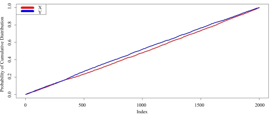
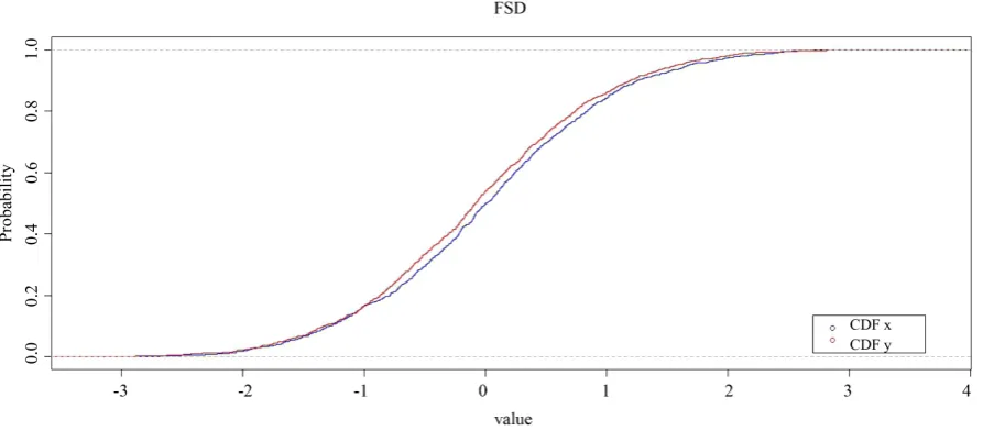
h , then X FSD Y. G: Test case.

Figure A1 plots the cumulative distributions for all observations of X and Y. The combined sorted vector doubles the length of observations, and thus distorts the image compared to the familiar CDF as plotted in Fig-ure A2 for each variable.

We can see in Figure A1 & Figure A2 the multiple crossing of the CDFs (around the 300th observation and −1 value respectively), thus negating any first degree stochastic dominance between variables. Clearly though, on balance we can see F X

( )

is more desirable than F Y

( )

.

For three h values (−0.99, −0.98, and −0.97) F_X

( )

h >F_Y

( )

h . Outside of those values, F_X

( )

h <F_Y

( )

h . This is where second degree stochastic dominance may offer some insight…

3) Module 3: Second Degree Stochastic Dominance (SSD)

B: Create an output vector to store the instances of area inequality.

[image:8.595.90.540.507.699.2]

C: Uses the sorted X and Y variables as the LPM target under n = 1. Thus all observations are used in the

(9)

[image:9.595.92.539.87.288.2]

113

Figure A2. Typical CDF plot for variables X and Y.

stringent “for all h” qualification. If

∫

_−∞h

(

h−X

) ( )

dF X <

∫

_−∞h

(

h Y−

) ( )

dF Y for that observation target h, no instance is recorded into the output vector (output_x[i] < −0). Conversely, if

(

) ( )

d

(

) ( )

d

h h

h X F X h Y F Y

−∞ − > −∞ −

∫

for that observation target h, the loop is stopped.

D: Uses the same logic as (C) above, only tests the inverse area relationships

(

) ( )

d

(

) ( )

d

h h

h Y F Y h X F X

−∞ − < −∞ −

∫

.

E: Plots the cumulative areas of each variable.

F: Reads the output vectors. If the output vector has 0 instances of

∫

_−∞h

(

h−X

) ( )

dF X >

∫

_−∞h

(

h Y−

) ( )

dF Y , then X SSD Y.

G: Test case.

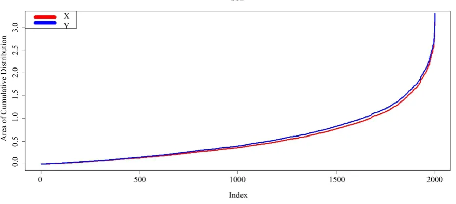
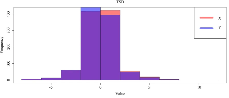
Figure A3 shows the cumulative distribution areas for X and Y. The lower area and thus dominance is quite

clear. Alternatively viewed as a histogram, Figure A4 illustrates

∫

_−∞h

(

h−X

) ( )

dF X >

∫

_−∞h

(

h Y−

) ( )

dF Y for all

positive values (a good thing), while simultaneously

∫

_−∞h

(

h−X

) ( )

dF X <

∫

_−∞h

(

h Y−

) ( )

dF Y for all negative values (also a good thing). This is evident when examining the skewness between both variables.

Skew(X) Skew(Y)

0.06529391 0.04430945

Nawrocki [4] also finds excess positive skewness for the risk averse investor’s portfolio compared to the maximum mean/variance portfolio. This in turn was expected, due to Hadar and Russell [3] original conclu-sions:

“For instance, we have indicated in the paper that FSD implies a certain relationship between the odd mo-ments (and sometimes also between the even momo-ments) of the prospects under consideration. Consequently, given that P is preferred to P’ for all monotonic utility functions, we can immediately say that all the odd mo-ments around zero of P are larger than the respective moments of P’.”

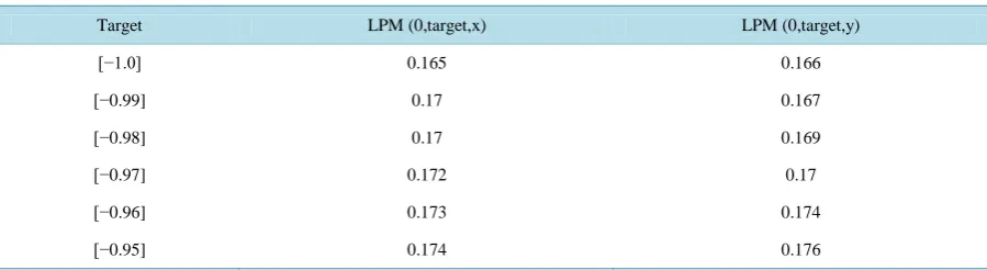
Even when dominance interruptions occur in the histogram, the cumulative area to that point is not enough to negate the dominance of X over Y. Revisiting the LPMs from the FSD interval of question tells a different story when areas are compared:

The areas in Table A1 never even really come close to intersecting like the CDFs did in Table A2. This result loosely supports the maximal hypothesis from Klecan et al. [11]—that the areas would have to be very volatile and crossing in order to negate SSD4, and if that were true, it would of course reflect on the underlying CDFs

(10)

[image:10.595.89.537.93.294.2]

Figure A3. Plot of h

(

h X

) ( ) (

dF X , h h Y

) ( )

dF Y

−∞ − −∞ −

[image:10.595.87.538.325.550.2]

∫

using all observations of X and Y as targets (h).

Figure A4. Histogram of h

(

h X

) ( ) (

dF X , h h Y

) ( )

dF Y

−∞ − −∞ −

[image:10.595.88.547.589.723.2]

∫

using all observations of X and Y as targets (h).

Table A1. Areas of variables X, Yover the interval [−1, −0.95].

Target LPM (0,target,x) LPM (0,target,y) LPM (1,target,x) LPM (1,target,y)

[−1.0] 0.165 0.166 0.0793658 0.0867652

[−0.99] 0.170 0.167 0.0810362 0.0884257

[−0.98] 0.170 0.169 0.0827362 0.0901005

[−0.97] 0.172 0.170 0.0844422 0.0917979

[−0.96] 0.173 0.174 0.0861641 0.0935241

(11)

[image:11.595.87.537.99.222.2]

115

Table A2. CDF values for different targets for variables X and Y.

Target LPM (0,target,x) LPM (0,target,y)

[−1.0] 0.165 0.166

[−0.99] 0.17 0.167

[−0.98] 0.17 0.169

[−0.97] 0.172 0.17

[−0.96] 0.173 0.174

[−0.95] 0.174 0.176

used in FSD.

4) Module 4: Third Degree Stochastic Dominance (TSD)

B: Create an output vector to store the instances of (area of the cumulative distribution)2 inequality.

C: Uses the sorted X and Y variables as the LPM target under n = 2. Thus all observations are used in the

stringent “for all h” qualification. If

∫

_−∞h

(

h−X

)

2dF X

( )

<

∫

_−∞h

(

h Y−

)

2dF Y

( )

for that observation target h, no instance is recorded into the output vector (output_x[i] < −0). Conversely, if

(

)

2

( )

(

)

2

( )

d d

h h

h X F X h Y F Y

−∞ − > −∞ −

∫

for that observation target h, the loop is stopped.

D: Uses the same logic as (C) above, only tests the inverse area relationships

(

)

2

( )

(

)

2

( )

d d

h h

h Y F Y h X F X

−∞ − < −∞ −

∫

.

E: Plots the cumulative areas squared for each variable.

F: Reads the output vectors. If the output vector has 0 instances of

∫

_−∞h

(

h−X

)

2dF X

( )

>

∫

_−∞h

(

h Y−

)

2dF Y

( )

, then X TSD Y.

G: Test case.

Figure A5 shows the TSD cumulative distribution areas for X and Y. The lower area and thus dominance is

quite clear. Alternatively viewed as a histogram, Figure A6 illustrates

∫

_−∞h

(

h−X

)

2dF X

( )

>

∫

_−∞h

(

h Y−

)

2dF Y

( )

for all positive values (a good thing), while simultaneously

∫

_−∞h

(

h−X

)

2dF X

( )

<

∫

_−∞h

(

h Y−

)

2dF Y

( )

for all negative values (also a good thing).

A.2. Generalized Stochastic Dominance Efficient Sets

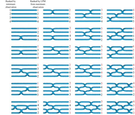
To extend the stochastic dominance tests and examine multiple portfolios, we use inspiration from Braid Theory. Braid Theory is an abstract geometric theory studying the everyday braid concept and we envision the CDFs as strings in these braids. Braids will nullify SD and avoid placing the CDFs in the “Dominated Set”. Figure A7

provides a visual representation of CDFs to braids, highlighting the crossing of CDFs the stochastic dominance routine is designed to decipher.

By testing for SD using the final ranks for that SD degree, we can derive the SD efficient sets. If a portfolio is dominated by a higher final ranked one, it is out of the efficient set. Example in Row 5 Column 4:

• The highest final ranked portfolio is the “Base”. Test the “Base” portfolio against the next highest ranked, the “Challenger”. 4 v 2. No SD exists. 2 joins the “Current Base” vector to run unidirectional5 SD tests from. • Test the new “Base” against the next “Challenger”. 2 v 3.2 SD 3. 3 is placed in the “Dominated Set”.

• Test the new “Base” against the next “Challenger”. 2 is the last entry in the “Current Base”. 2 v 1. No SD

5_{The earlier discussed tests were bi-directional, which involves more calculations between variables. Since the efficient sets are determined}

(12)

[image:12.595.89.539.90.278.2]

116

Figure A5. Plot of ( )2d ( ) (, )2d ( )

h h

h X F X h Y F Y

−∞ − −∞ −

∫

using all observations of X and Y as targets (h). Note the effects of

the higher loss aversion (n) on the distribution versus SSD cumulative plot in Figure A3.

Figure A6. Plot of ( )2 ( ) ( )2 ( )

d , d

h h

h X F X h Y F Y

−∞ − −∞ −

∫

using all observations of X and Y as targets (h). Note the effects of

the higher loss aversion (n) on the distribution versus the SSD histogram in Figure A4.

exists. Test the remaining “Current Base” vector against 1. 4 v 1. No SD exists, 1 joins the “Current Base”. • There are no more “Challengers”. Stop the procedure. The SD efficient set is the final ranked set less the

“Dominated Set” {4,2,1}.

• #1 (the largest minimum value) can never be dominated, thus it is in every efficient set.

This procedure is different than that proposed by Porter, Wart and Ferguson [12] in several regards. One dif-ference is that we do not check multiple SD degrees simultaneously6. Our second difference is we determine the final ranking by ordering the LPMs from the maximum of all observations. We substitute the degree 1 LPM fi-nal ranking for Porter et al.’s use of means and variances in ranking the securities. Finally, our third difference is the integration of the “Tricks” Porter et al. [12] identified to reduce the computational burden. We use the min-imum value check as an “if” condition (“Trick 1”); and {break} commands at the end of each observation if a “Base” falls behind the “Challenger”.

[image:12.595.89.539.326.520.2]

(13)

[image:13.595.74.538.88.484.2]

117

Figure A7. SD efficient sets (in red), versus ranked securities or portfolios in ascending order by their LPM from the

maxi-mum observation across all variables.

(14)

Appendix C

R CODE

This section of the paper will provide the R code for the stochastic dominance test using lower partial moments. 1) Module 1: Lower Partial Moment Function (LPM)

(15)

119

(16)

(17)

121

(18)

(19)

(20)

(21)

(22)