http://dx.doi.org/10.4236/gep.2016.43005
Using a Coupled Air Quality Modeling
System for the Development of an Air
Quality Plan in Madrid (Spain): Source
Apportionment and Analysis Evaluation
of Mitigation Measures
Raúl Arasa1, Anna Domingo-Dalmau1, Ricardo Vargas2
1Technical Department, Barcelona, Spain
2Environmental and Territorial Planning Agency, Regional Government of Madrid, Madrid, Spain
Received 16 February 2016; accepted 15 March 2016; published 18 March 2016
Copyright © 2016 by authors and Scientific Research Publishing Inc.
This work is licensed under the Creative Commons Attribution International License (CC BY).
http://creativecommons.org/licenses/by/4.0/
Abstract
Keywords
Environmental Assessment, Air Quality Modelling, CMAQ, Emissions, Madrid, Air Quality Plan, Mitigation Measures
1. Introduction
The largest amount of gases and aerosols emitted into the atmosphere are generated in cities with poor land ex-tension and large population (about 50% population in 0.1% land area). These emissions influence weather and climate [1] and health. Recently, pollution has been included as one of the cancer-causing agents by the World Health Organization [2]. Even pollutant concentrations remain high, particularly in urban areas, air emissions have been reduced significantly in recent years [3]. Road traffic emissions associated with combustion and road dust resuspension processes are the main causes of pollution in urban areas and conurbations [4]-[7].
In these areas, there are high levels of nitrogen dioxide (NO2) and particulate matter (PM10) by comparison with the air quality standards (European Directive EC/2008/50). In Spain, annual average values of NO2 and PM10 are elevated in many urban air quality measurement stations with traffic influence [8]. Whereas, high ozone levels are measured in rural or suburban areas located downwind of urban or industrial locations and where local ozone precursors are lacking [9] [10]. Scientific studies has demonstrated that exposure to a high levels of NO2, O3 or PM10 can increase respiratory problems as inflammation, can lead to asthmatic responses in sensitive people or even cause premature death [11]-[15].
In order to improve air quality levels in urban areas, in the last years they have been developed international and national action plans [16]-[18]. Policies over traffic sector to improve air quality in urban areas have fol-lowed different strategies associated: to decrease variables associated with traffic which directly affect the amount of pollutant emissions (velocity or intensity vehicles flow); and to change Vehicles Park distribution, to introduce new technologies or alternative fuels [19] [20].
In the same way, Madrid has developed an ambitious action plan to improve the air quality in the last years. Previously to the development of the air quality plan evaluated in this paper, the Regional Government of Ma-drid developed the Air Quality and Climate Change Strategy 2006-2012 (Plan Azul). This plan established an amount of 111 measures with a degree of compliance of 87%. Furthermore, the Regional Government of Madrid updates periodically its emission inventory (14 versions in the last 24 years), and considers air quality modelling to evaluate mitigation measures prior to adopting them.
In this sense, air quality modelling has become a useful tool for administrations since it provides them a me-thod to deal with human resources, production, emergency proceedings or to improve existing air quality plans and test abatement strategies. In the last years, local administrations have used models to prepare air quality plans in urban areas as the Plan Azul case. Models are able to provide the difference of pollutants concentration and a quantitative assessment of the effect of policies and mitigation plans [21]-[27].
This work aims to investigate the effect on air quality concentrations of measures proposed by the air quality plan called Air Quality and Climate Change Strategy of the Regional Government of Madrid 2013-2020 (Plan Azul +). Specifically, we will analyze one scenario with all measures proposed applied over emissions inventory, affecting traffic, residential and industrial sectors (section 2.3). The study includes a numerical deterministic evaluation that shows the accuracy of the air quality modelling outputs; and a source apportionment analysis to know the contribution to air quality levels of each emission sector.
We have used WRF-ARW/AEMM/CMAQ (Section 2.2) modelling system to evaluate the impact of each emission scenario by sensitive analysis (comparison between scenarios). To develop this air quality modelling system, we have followed the recommendations proposed by [28] on the Guide on the use of models for the Eu-ropean Air Quality Directive.
Description of the modelling system used, is presented in Section 2, as well as the area characteristic, data used, episode selection and mitigation measures proposed. A detailed analysis of the results obtained is pre-sented in Section 3, and finally, some conclusions are reported in Section 4.
2. Methodology
pe-riod analyzed, the action plans considered and their corresponding scenarios is included below.
2.1. Area Characteristic, Data Used and Episode Selection
The area of study has been Madrid in the centre of the Iberian Peninsula over the Central Plateau. The Commu-nity of Madrid is surrounded by the autonomous communities of Castile and León and Castile-La Mancha and covers the 1.6% percent of the territory of Spain. Madrid and its metropolitan area is the third-largest in the Eu-ropean Union and due to its economic activity, high standard of living, and market size, is considered one of the major financial centre of Southern Europe. Madrid is served by highly developed communication infrastructures and one of the regions best connected by roads and railways in Europe.
The population of Madrid metropolitan area reached in 2012 a population of 6.5 million (around 14% of Spain). The Community of Madrid is composed on 179 municipalities, being Alcalá de Henares, Alcobendas, Alcorcón, Fuenlabrada, Getafe, Leganés, Madrid, Móstoles, Parla and Torrejón de Ardoz the most populated. Madrid is the capital and largest city in Spain.
Madrid presents a varied topography combining mountain peaks rising above 2000 m, holm oak dehesas and low lying plains, being 650 meters the average altitude. Peñalara is the highest mountain in Madrid, reaching 2428 m.a.s.l., located in the Guadarrama mountain range in the west region of the Community.
Since a climate point of view Madrid has a temperate Continental Mediterranean climate with cold winters with temperatures below 0˚C habitually. During summer temperatures rises above 30˚C and frequently reach 40˚C in July. Yearly average precipitation levels are below 500 mm, distributed throughout the year and with maximums in autumn and spring. Hottest and driest regions are reproduced in the flatter areas on the south of the region, whereas coldest and wettest areas are located in the mountain ranges. In the urban areas of Madrid the climate is modified by the heat island effect, increasing mainly nocturnal temperatures.
Anthropogenic contribution dominates pollutant air emissions in Madrid. Transport emissions (road and non-road traffic) from the metropolitan area of Madrid are the main CO, NOx and particulate matter emission sector, representing between a 53 and an 86% of the total emissions. Airport represents a important contribution to the emissions of the whole Community of Madrid. On other hand, industrial emissions dominate SOx and NMVOCs (non-methane volatile organic compounds) emissions.
In Figure 1, we show models domains used for simulations (Section 2.2) that represents the Community of
Madrid.
Regarding the air quality levels, ozone and nitrogen dioxide limit values fixed by the European Air Quality Directive EC/2008/50 has been exceeded during the last years. In 2010, the O3 threshold information value was exceeded in 30 occasions in the air quality stations handled by the Regional Government of Madrid. NO2
[image:3.595.91.538.485.695.2]
maximum 1-hour limit value was exceeded in 31 occasions but not exceeding the tolerance fixed by the Direc-tive (18 occasions permitted per year and station). In the recent years SO2 and PM10 levels have showed a de-crease, whereas O3 has showed a trend to rise. The rest of pollutants remain constants with exceedances of the NO2 annual limit value.
To realize this study we have chosen 2010 as modelling year. The whole calendar year has been considered to analyze the source apportionment of every emission sector, and 10 meteorological episodes of 48 hours in 2010 have been considered to evaluate each mitigation measure. We have selected meteorological episodes with the highest NO2 and O3 concentrations measured, evaluating mitigation scenarios in the worst case since an air qual-ity point of view. 5 meteorological episodes correspond on highest O3 concentration and 5 on highest NO2 con-centration.
[image:4.595.89.534.290.723.2]We have characterized episodes using air quality measurements from the Air Quality Network that belongs to the Environment and Territorial Planning Agency of the Regional Government of Madrid. In Table 1, we show the date of every episode selected, NO2 and O3 maximum 1-h per episode and annual average of these statistics.
Table 1. NO2 and O3 daily maximum 1-h values measured in the air quality stations of the Community of Madrid during meteorological episodes selected and annual average (U correspond to urban station; S, suburban; R, rural; T, traffic; I, in-dustrial; and F, background).
Air Quality Station
Period and NO2 daily maximum 1-h (µgm−3) Period and O3 daily maximum 1-h (µgm−3)
17/03 20/10 28/10 04/11 28/12 Annual
average 24/06 06/07 08/06 11/08 20/08 Annual average
Alcalá de Henares (UT) 68 129 119 97 161 68 151 164 100 194 159 93
Alcobendas (UI) 131 174 134 156 172 67 148 181 70 163 153 82
Alcorcón (UF) 141 186 179 188 135 80 135 154 72 141 139 86
Algete (SF) 68 69 79 53 50 34 166 186 105 175 168 102
Aranjuez (UF) 50 113 127 104 74 55 109 103 81 130 144 81
Arganda del Rey (UI) 82 75 79 50 63 45 85 133 81 178 119 78
Colmenar Viejo (UT) 129 155 168 118 131 82 135 139 91 98 150 85
Collado Villalba (UT) 209 233 153 163 149 75 155 174 95 165 174 90
Coslada (UT) 112 84 217 202 188 101 130 139 69 177 150 78
El Atazar (RF) 4 13 100 6 49 11 171 171 106 134 153 104
Fuenlabrada (UI) 168 -- 154 175 114 82 122 143 67 138 121 79
Getafe (UT) 96 200 219 234 126 82 130 131 79 124 127 76
Guadalix de la Sierra (RF) 43 45 63 31 58 26 85 183 80 148 170 92
Leganés (UT) 158 133 147 149 157 93 118 123 46 145 134 75
Majadahonda (SF) 145 144 121 155 144 67 153 181 95 139 152 95
Móstoles (UF) 149 126 129 139 135 71 73 114 87 104 -- 77
Orusco de Tajuña (RF) 4 31 25 29 23 13 148 138 116 219 144 102
Rivas Vaciamadrid (SF) 102 148 159 130 121 79 124 134 89 160 137 84
San Martín de Valdeiglesias (UF) 48 34 42 32 54 20 118 137 108 143 150 89
Torrejón de Ardoz (UF) 82 150 172 123 88 58 113 97 83 138 137 76
Valdemoro (SF) 98 84 89 77 87 56 124 125 67 153 133 84
Villa de Prado (RF) 36 32 64 11 56 18 130 119 96 89 126 85
2.2. Modeling Approach and Emissions Inventory Used
The design, implementation and configuration of the air quality modelling system have been made by research-ers with an extensive experience as modellresearch-ers [29] [30]. The air quality modelling system has been set with the optimum parameterizations to reduce the uncertainty of the models [31]-[33]. The authors have applied this kind of models as forecast tool as assessment tool of mitigation plans [26] working in collaboration with different re-gional and local administrations (Environmental and Water Agency of Andalusia Government, Environment and Territorial Planning Agency of Regional Government of Madrid and Territory and sustainability Agency of Cat-alan Government).
Three models compose the air quality modelling system: a meteorological model, an emission model and a photochemical model. The recommendations and requirements indicated in the Guide on the use of models for the European Air Quality Directive [28] have been used for the models configuration, and also to choose the op-timum kind of models used to evaluate the air quality plans. This coupled air quality modelling system has been applied and tested successfully in urban, industrial and mine areas. Urban areas as Madrid, Barcelona, Seville (Spain) or Nice (France); industrial areas as Ponferrada or Tarragona (Spain); and mine areas as Calama (Chile). The air quality modelling system showed has been evaluated using Maximum Relative Directive Error [28] re-ferred in the European Directive EC/2008/50. Results obtained from this evaluation accomplish the model un-certainty limits according to the Directive for the pollutants O3, NO2, PM10, SO2 and CO, having used measure-ments from more than 120 stations (urban, suburban and rural locations) during a period of four years. In section 3.1 we show the evaluation of the air quality modelling system developed in the region of Madrid.
The following paragraphs outline the main features of the three models which compose the modelling system.
2.2.1. Meteorological Model
The mesoscale meteorological model used is Weather Research and Forecasting—Advanced Research (WRF- ARW) version 3.3 [34]. WRF model was configured with four nested domains with 27 (first domain), 9 (second domain), 3 (third domain) and 1 km (fourth domain) of horizontal resolution (Figure 1). First domain, called d01, covers the southwest of Europe and the north of Africa with 108 × 97 grid cells. Second domain (d02), covers the whole of the Iberian Peninsula with 142 × 118 cells. And the inner domains cover the Community of Madrid (d03 with 52 × 55 cells) and the city of Madrid and its metropolitan area (d04 with 61 × 43 cells). The vertical resolution includes 32 levels, 22 below 1500 meters, with the first level at approximately 15 meters and the domain top at about 100 hPa. The vertical structure covers the whole troposphere and a resolution decreasing slowly with height in order to allow low-level flow details to be captured. The higher resolution close to the surface is a common practice in air quality studies in order to better represent the physical-chemical processes within the Atmospheric Boundary Layer [35]-[38]. Initial and boundary conditions for domain d01 were sup-plied by the National Center for Environmental Prediction and National Center for Atmospheric Research (NCEP/NCAR) Climate Forecast System Reanalysis with 0.5˚ of spatial resolution and 6 hours of temporal sampling. We use a WRF physical configuration used in preliminary studies [26] that provides good results for air quality applications in the Iberian Peninsula [39]. Two-way nesting is used as relationship between domains for the three external domains (D01, D02 and D03) and one-way nesting for D04 due to computational issues.
2.2.2. Emission Model
inventory version 2010 includes emissions classified by Selected Nomenclature for Air Pollution (SNAP) sec-tors (Table 2). Additionally, we use bottom-up methodology to calculate natural emissions for d02, d03 and d04 domains. As natural emissions we consider those caused by vegetation [42] or erosion dust [43] using paramete-rizations, land uses and meteorological outputs from WRF. These emissions are adapted and speciated by AEMM model to the requirements of the chemical module of CMAQ.
AEMM model also includes an emission projections module called AEMM-EP. This module estimates future emissions in the Community of Madrid. AEMM-EP does not realize a specific forecast, according with consid-erations of the EMEP/EEA emission inventory guidebook 2013 [44]. Projections are a tool to assess what might happen it we take no action, what might be achieved with actions we are committed to and what else could be done (EMEP/EEA 2013). Projections importance lies in considering different developments in the economy, technologies or policies for a sustainable development. In this way, projections are a tool to know what happens to the amount of atmospheric emissions without considering mitigation measure, with measures already taken, and considering further actions.
2.2.3. Photochemical Model
The U.S. Environmental Protection Agency models-3/CMAQ model is the one used to simulate the physical and chemical processes into the atmosphere [45]. CMAQ is an open-source photochemical model which is updated periodically by the research community. In this contribution we use CMAQv4.7.1, considering CB-5 chemical mechanism and associated EBI solver [46] and AERO5 aerosol module [47]. Regarding atmospheric chemistry, CB5 considers 155 chemical reactions that involve NOx, non-methanic volatile organic compounds (NMVOCs) or ozone (O3). Additional details regarding the latest release of CMAQ can be found on the Community Model-ling and Analysis System (CMAS) Center (www.cmascenter.org). CMAQ model uses the same configuration as the WRF simulation. Initial and boundary conditions for d02 domain are provided by the results of simulation of d01 domain. And the same relationship is followed between d02 and d03, d03 and d04. Meteorology-Chemistry Interface Processor (MCIP) version 3.6 is used to prepare WRF output to CMAQ model. And AEMM model prepares emissions as AERO5 and CB5 modules require.
The whole year 2010 has been modelled with simulations of 48 hours of duration for every day of the year. In order to minimize the effects of the initial conditions, the first 24 hours of each simulation have been discarded as they have been considered as spin-up time.
[image:6.595.85.537.485.722.2]The air quality modelling simulations have run in Meteosim’s computing cluster, which has 27 nodes and more than 212 cores.
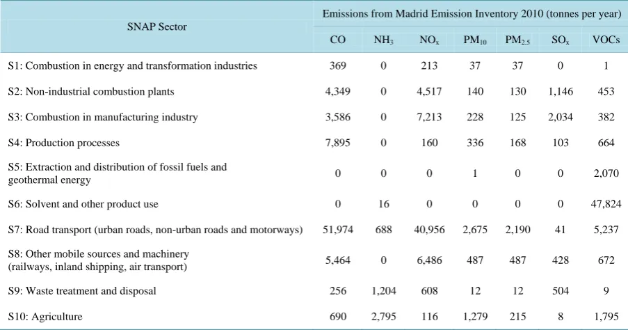
Table 2.SNAP sectors considered into the Madrid Emission Inventory and their pollutant emissions.
SNAP Sector
Emissions from Madrid Emission Inventory 2010 (tonnes per year)
CO NH3 NOx PM10 PM2.5 SOx VOCs
S1: Combustion in energy and transformation industries 369 0 213 37 37 0 1
S2: Non-industrial combustion plants 4,349 0 4,517 140 130 1,146 453
S3: Combustion in manufacturing industry 3,586 0 7,213 228 125 2,034 382
S4: Production processes 7,895 0 160 336 168 103 664
S5: Extraction and distribution of fossil fuels and
geothermal energy 0 0 0 1 0 0 2,070
S6: Solvent and other product use 0 16 0 0 0 0 47,824
S7: Road transport (urban roads, non-urban roads and motorways) 51,974 688 40,956 2,675 2,190 41 5,237
S8: Other mobile sources and machinery
(railways, inland shipping, air transport) 5,464 0 6,486 487 487 428 672
S9: Waste treatment and disposal 256 1,204 608 12 12 504 9
2.3. Modeling Scenarios
In the following lines, we explain the modelling scenarios defined and the methodology used to evaluate them.
2.3.1. Source Apportionment
The first analysis realized is a source apportionment exercise. The aim of this analysis is to obtain the contribu-tion to the air quality levels of the different emission sector. To accomplish with this goal a zero-out methodol-ogy was followed, also know as the brute force method or as single-perturbation method [48] [49]. The applica-tion of this methodology consists on the comparison between the results of the air quality modelling system ex-ecuted considering all emission sectors regarding the results obtained by the same system turning off one source of emissions. Turning off a specific sector is equivalent to reduce a 100% (zero-out) its emission value. This ap-proach lets to isolate the response in nonlinear systems. In our case, we have realized nine modelling different scenarios turning off sectors. We have turned off snap sectors and to simplify we have considered S3, S4 and S6 as an only one sector (called S346). Additionally, we have turned off natural emissions included in the model-ling system.
2.3.2. Mitigation Measures Effect
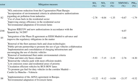
The second analysis focus on the evaluation of mitigation measures over the air quality levels. We take into ac-count mitigation measures considered in the Air Quality and Climate Change Strategy of the Regional Govern-ment of Madrid 2013-2020 (Plan Azul +). More information about Plan Azul + can be found at the official en-vironmental webpage of the Community of Madrid. In Table 3, we show mitigation measures considered and their effect over atmospheric emissions for the Community of Madrid as a whole. Mitigation measures defined in the Plan are focused on the reduction of NO2 levels primordially. For this reason we focus our attention on the effect of the Plan over NO2 and O3.
[image:7.595.93.538.451.716.2]Previously to analyze the combined effect of all mitigation measures considered in Table 3, individualized analysis was realized for different strategic measures. Considering the results obtained, some measures were ac-cepted or modified or denied. Measures finally planned and acac-cepted were those that good results were found in terms of reduction of air quality levels.
Table 3. Mitigation measures classified by SNAP sectors and their emission reduction estimation in comparison with the base case scenario.
Sector Mitigation measure SOx
(%) NOx (%) CO (%) NMVOCs (%) PM10 (%) S2 *NO
2 emissions reduction from the Cogeneration Plant Barajas *Incorporation of environmental criteria in administrative authorizations
regarding air pollution from industries *
Use of clean fuels in the residential sector
*Improving energy efficiency in the residential sector
*Environmental adaptation of livestock farms
−2.78 −8.04 −1.35 −0.67 −1.79
S346 *
Register RIECOV and new authorizations in accordance with the
Spanish lay 34/2007 −6.07
S5 *
Integration of the Phase II agreement as EESS Madrid to advance and
improve the regulatory obligations in the matter −3.66
S7
*Renewal of the fleet autotaxi fuels and clean technologies
*Public-private partnership to promote the use of gas vehicles collaboration
*Implementation and consolidation of charging infrastructure and
encouraging the use of electric vehicles *
Renewal of institutional fleet under environmental criteria *Urban and inter-city buses cleaner
*Renewal the vehicles park with more efficient models
*Low emission zones and residential areas of priority
*Circulation efficient vehicles by BUS HOV lanes
*To promote gas fuel for duty vehicles in the corridor Madrid—
Castile La Mancha—Valencia
−5.93 −7.15 −2.19 −2.76 −8.30
S8
*Implementation of the AENA agreement in Barajas.
As [28] recommends sensitivity analysis has been made in order to evaluate the results obtained by the Air Quality Modelling system considering Plan Azul + emissions. The basis of a sensitivity analysis is to compare the results obtained in the real scenario versus the results obtained modifying the emissions. These emission variations result from the implementation of mitigation measures. The reduction of pollutant concentrations can directly be determinate using this approach.
3. Results and Discussion
In the following subsections we present a evaluation of the air quality modelling system, the source apportion-ment analysis realized, the effect of mitigation measures defined in the Plan Azul + over air quality levels, and the emission projections for 2020.
3.1. Air Quality Modeling Evaluation
Two evaluations have been realized to evaluate the accuracy of the air quality modelling system designed and developed. By one hand, we have used the uncertainty definition for modelling of the European Directive EC/2008/50, and on the other hand, we have realized a numerical deterministic evaluation. Twice evaluations have been developed for the whole 2010 year.
As European Directive suggests, models must be verified and validated before they can be used for air quality assessment or management [28]. The quality objectives for a model are given as a percentage uncertainty. The definition of the uncertainty of the models is ambiguous in the Directive. Since values may be calculated, a ma-thematical formula would have made the meaning much clearer, as such, the term “model uncertainty” remains open to interpretation. Despite this, [28] suggests that it should be called the Relative Directive Error (RDE) and defines it mathematically at a single station as follows:
LV LV
O M
RDE
LV
−
= (2)
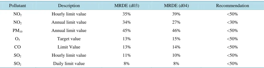
where OLV is the closest observed concentration to the limit value (LV) or the target value for ozone and MLV is the correspondingly ranked modelled concentration. The maximum of this value found at 90% of the available stations is then the Maximum Relative Directive Error (MRDE). MRDE values and Directive recommendations are showed on Table 4. Results indicate that model uncertainty requirement is achieved for all pollutants and so, the air quality modelling system presented in this paper can be used for the aims the Directive considers.
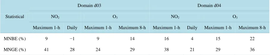
[image:8.595.87.539.603.720.2]Statistical metrics for photochemical model performance assessment are calculated for surface ozone and ni-trogen dioxide concentrations at 23 measurement stations (Table 1). We consider NO2 and O3 because mitiga-tion measures are focused on the reducmitiga-tion of these atmospheric pollutants. The two multi-site metrics used are the mean normalized bias error (MNBE) and the mean normalized gross error (MNGE). The U.S. Environmen-tal Protection Agency [50] developed a guideline indicating that it is inappropriate to establish a rigid criterion for model acceptance or rejection. However, building on past air quality modelling applications [51] common values ranges have been established [29]. The accepted criteria are MNBE, ±5 to ±15%; and MNGE, +30 to +35%. For the entire period studied (2010), the results in Table 5 show the statistics metrics of daily maximum 1-h and 8-h values for O3 and maximum 1-h and daily values for NO2.
Table 4.MRDE values calculated using the air quality modelling system predictions taking into account the whole 2010 year.
Pollutant Description MRDE (d03) MRDE (d04) Recommendation
NO2 Hourly limit value 35% 39% <50%
NO2 Annual limit value 34% 27% <30%
PM10 Annual limit value 45% 46% <50%
O3 Target value 13% 15% <50%
CO Limit Value 13% 14% <50%
SO2 Hourly limit value 11% 10% <50%
Table 5. MNBE and MNGE statistical values corresponding to NO2 and O3 concentrations for the domains d03 and d04.
Statistical
Domain d03 Domain d04
NO2 O3 NO2 O3
Maximum 1-h Daily Maximum 1-h Maximum 8-h Maximum 1-h Daily Maximum 1-h Maximum 8-h
MNBE (%) 9 −1 9 14 16 4 15 22
MNGE (%) 41 28 24 29 38 21 29 36
Results indicate that the model shows a clear tendency to overestimate ground level ozone and NO2 concen-tration, being MNBE positive in the major part of the cases. Ozone prediction shows a better accuracy than NO2 forecast. NO2 worst values are obtained for measurement stations located in rural areas (Algete, Orusco de Ta-juña or Villa de Prado), whilst the best results are obtained in urban stations like Alcorcón, Leganés or San Martín de Valdeiglesias. The opposite result is obtained for the ozone evaluation: best results in rural areas (El Atazar, Orusco de Tajuña or Villarejo de Salvanés) and worst results in urban stations (Coslada, Arganda del Rey or Móstoles). These results show that the model predicts better NO2 and O3 in locations where measured levels of each one of these pollutants are higher. Analyzing the daily profile of ozone, we have observed a typi-cal overestimation during the night. This fact can be associated to the model does not represent nocturnal physi-cochemical processes accurately enough [52] or night-time emissions profile. To solve this problem often evalu-ation statistics are calculated using only the hourly observevalu-ation-predictions pairs for which the observed concen-tration is greater than a specific value [29]. We have used 60 µgm−3 as cut-off value [53]-[55] and when we ap-ply this restriction, reductions of 9% (maximum 8-h) and 13% (maximum 1-h) have been obtained. In the same way for NO2 concentrations we have eliminated very low concentrations, and a cut-off of 25 µgm−3 has been de-fined. The application of this restriction improves forecast between a 12% - 15%. The correlation coefficient evaluated using maximum 1-h value is 0.7 for ozone concentration (d03 and d04) and 0.8 and 0.9 for NO2 con-centration (d03 and d04 respectively).
3.2. Source Apportionment Analysis
The emission inventory values showed on Table 2 provides that traffic sector (S7) is the main responsible to the emissions of the whole region of Madrid for CO (59% of contribution), NOx (68%), PM10 (47%) and PM2.5 (60%), whilst S346 is the main for SO2 (73%) and NMVOCs (89%). As we have commented previously we have followed a zero-out methodology to realize the source apportionment analysis for the air quality levels us-ing CMAQ photochemical model.
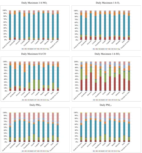
In Figure 2, we show the contribution of the different snap sectors and natural contribution (calculated using AEMM model) to the levels of NO2, O3, CO, SO2, PM10 and PM2.5 using different statistical daily values.
As we could expect traffic sector is the main responsible to NO2 levels with contributions between 73% - 89%. Second most important contribution corresponds to other mobile sources, airport mainly, with up to a 12% in some municipalities. For this pollutant agriculture is a relevant sector in municipalities away the urban metro-politan area of Madrid. In the case of ozone, again traffic sector is the main contributor with a percentage be-tween 57% - 77%. Other mobile sources and non-industrial combustion plants are the second and the third con-tributor sector, respectively, with values between 7% - 19% and 7% - 12%. CO results are very similar than those obtained for O3 with a most relevant contribution of S346 sector in some municipalities (Getafe and Le-ganés) more industrialized. PM10 and PM2.5 main contributor is traffic sector (33% - 59%). In comparison with NO2 or O3 the percentage is lower and the relevancy of the other sectors is higher. Agriculture affects an 11% - 36%, being most important for PM10 than PM2.5; and S346 provides a percentage of 8% - 21% to the particulate matter levels. Finally, the distribution of SO2 contributors is different, being S2 (Alcorcón 61% and Móstoles 55%), S346 (Alcalá de Henares 39%) or S8 (Alcobendas 43% and Coslada 48%) the main contributors to the air quality levels.
Daily Maximum 1-h NO2 Daily Maximum 1-h O3
Daily Maximum 8-h CO Daily Maximum 1-h SO2
[image:10.595.87.541.81.570.2]Daily PM10 Daily PM2.5
Figure 2.Contribution of the emission sectors (snap and natural) to the air quality levels for different municipalities in the region of Madrid.
3.3. Effect of Mitigation Measures over Air Quality Levels
As we can comment previously a sensitivity analysis has been made considering all mitigation measures of Ta-ble 3 and comparing with the results obtained in the base case. Real emissions (industry, traffic, natural, etc.) from the emission inventory are considered in the base scenario. In order to analyze the effect of the mitigation plan, the comparison has been made in some daily statistical values; focus our attention on NO2 and O3.
Geographically results are shown in the air quality zones of the region of Madrid
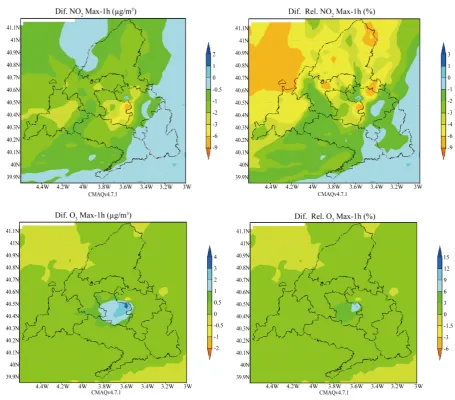
[image:11.595.83.539.80.480.2]
Figure 3.Difference (left) and relative difference (right) of daily maximum 1-h of NO2 (up) and O3 (bottom) between Plan Azul + scenario and base case scenario over the whole region of Madrid.
criterion, for this pollutants the results corresponds to the five periods defined in Table 1 (the effect of the miti-gation plan is analyzed during episodes while NO2/O3 levels are higher than the average annual value). In the rest of cases (PM10, PM2.5, CO and SO2), the results correspond to the average of ten periods defined in Table 1.
The effect of the mitigation plan directly results in a reduction of the levels of primary pollutants such as NO2. The highest nitrogen dioxide reductions are reached in Madrid city centre and around the big neighbour towns. The application of Plan Azul + mitigation plan reduces about 15% of nitrogen dioxide values in Madrid air qual-ity zone and Corredor del Henares air qualqual-ity zone; 9% in Cuenca del Alberche air qualqual-ity zone; 8% in Urbana Noroeste air quality zone; 7% in Urbana Sur air quality zone; and 3% in Cuenca del Tajuña air quality zone.
The comparison of the effect over NO2 hourly maximum values between base case scenario and Plan Azul + mitigation plan is showed in Table 6. We show mean and maximum difference corresponding to the average and the maximum of grid cell values for each air quality zone. NO2 hourly maximum values are reduced up to 11 µgm−3 in Madrid air quality zone, and up to 9 µgm−3 in Corredor del Henares air quality zone.
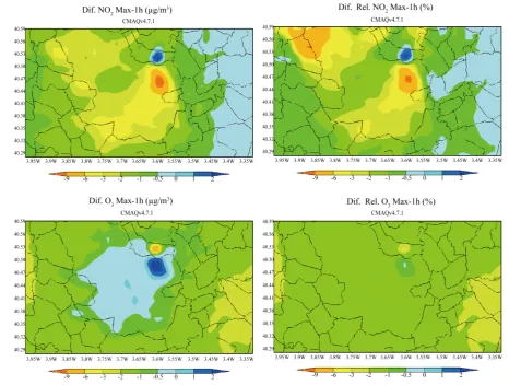
Figure 4. Difference (left) and relative difference (right) of daily maximum 1-h of NO2 (up) and O3 (bottom) between Plan Azul + scenario and base case scenario over the urban metropolitan area of Madrid.
Table 6.Effect of mitigation plans over NO2 1-h Maximum values in the Air Quality Zones.
Air Quality Zone NO2 Max. 1h (µgm−3) Mean Difference (µgm−3) Maximum Difference (µgm−3)
Madrid 76 −2.53 −11.30
Corredor del Henares 58 −1.24 −8.97
Urbana Sur 51 −0.92 −3.68
Urbana Noroeste 42 −1.37 −3.24
Sierra Norte 21 −1.03 −2.47
Cuenca del Alberche 30 −1.63 −2.75
Cuenca del Tajuña 24 −0.28 −0.69
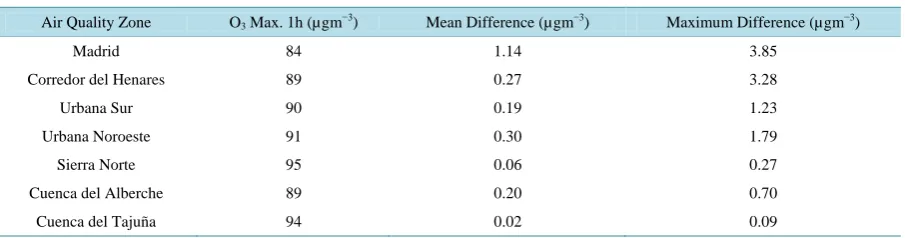
[image:12.595.90.539.482.623.2]Table 7. Effect of mitigation plans over O3 1-h Maximum values in the Air Quality Zones.
Air Quality Zone O3 Max. 1h (µgm−3) Mean Difference (µgm−3) Maximum Difference (µgm−3)
Madrid 84 1.14 3.85
Corredor del Henares 89 0.27 3.28
Urbana Sur 90 0.19 1.23
Urbana Noroeste 91 0.30 1.79
Sierra Norte 95 0.06 0.27
Cuenca del Alberche 89 0.20 0.70
Cuenca del Tajuña 94 0.02 0.09
mean and maximum difference corresponding to the average and the maximum of grid cell values for each air quality zone.
For the rest of pollutants the effect of the Plan is not so remarkable, with global reductions of CO, PM10, PM2.5 and SO2 lower than 5%. Anyway, we have identified that Plan Azul + have a local effect over these pol-lutants in specific locations as, for example, near the International Airport of Madrid, increasing the effect up to a 30%.
Using the modelling year 2010, we estimate that the application of the Plan could reduce the number of ex-ceedances of the hourly limit value of NO2 in a 20%, and the exceedances of PM10 in a 5%. Not changes in the number of ozone exceedances have been estimated.
4. Conclusions
A coupled air quality modelling system has been used for the design and preliminary evaluation of an air quality plan over a region with exceedances and high levels of atmospheric pollutants. The numerical modelling system accomplishes with the European Directive requirements and its accuracy is good enough as to use for evaluate air quality plans and mitigation measures. Results of evaluation also show that the system provides high accura-cy over locations with higher levels of NO2 and O3.
Results obtained show that the main sector contributor to the emissions and air quality levels over Madrid is the road traffic, followed for other mobile sources and non-industrial combustion plants as second and third contributors respectively. Moreover, air quality levels are determined basically for local contributions in Madrid and its urban metropolitan area. In this way, mitigation measures designed and evaluated have been focused on this sector.
We have observed that the Plan designed is optimum to reduce NO2 levels, reducing up to 11 µgm−3 the con-centration over the city of Madrid. Highest reductions of this pollutant are located over urban areas with traffic influence, coinciding with regions where NO2 levels traditionally are higher. The air quality plan has the effect with opposite sign and provides slight increases of ozone concentration (1% - 2%) in areas with typically ozone levels which are low. We expect that the application of this Plan will reduce the number of exceedances of the NO2 limit value and not affects considerably to the number of exceedances for ozone. Mitigation measures de-fined in the plan do not affect remarkably to the levels of CO, SO2 or particulate matter.
Acknowledgements
This work was funded by the Government of Madrid (Consejería de Medio Ambiente y Ordenación del Territo-rio) through the project “Definición, implementación y seguimiento de la Estrategia de Calidad del Aire y Cam-bio Climático de la Comunidad de Madrid 2013-2020” and by the Spanish Government through PTQ-12-05244. The authors gratefully acknowledge the technicians at the regional Environmental Agency of Madrid for pro-viding local information and emissions inventory and NOVOTEC consultants for their support and collabora-tion.
References
[2] Straif, K., Cohen, A. and Samet, J. (2013) International Agency for Research on Cancer (IARC). IARC Scientific Pub-lication No. 161: Air pollution and Cancer, Worlh Health Organization.
[3] EEA Report. No. 9/ 2913. Air Quality in Europe—2013 Report. http://www.eea.europa.eu/publications/air-quality-in-europe-2013
[4] Colvile, R.N., Hutchinson, E.J., Mindell, J.S. and Warren, R.F. (2001) The Transport Sector as a Source of Air Pollu-tion. Atmospheric Research, 35, 1537-1565. http://dx.doi.org/10.1016/S1352-2310(00)00551-3
[5] Anttila, P., Tuovinen, J.-P. and Niemi, J.V. (2011) Primary NO2 Emissions and Their Role in the Development of NO2 Concentrations in a Traffic Environment. Atmospheric Environment, 45, 986-992.
http://dx.doi.org/10.1016/j.atmosenv.2010.10.050
[6] Amato, F., Pandolfi, M., Alastuey, A., Lozano, A., Contreras, J. and Querol, X. (2013) Impact of Traffic Intensity and Pavement Aggregate Size on Road Dust Particles Loading. Atmospheric Environment, 77, 711-717.
http://dx.doi.org/10.1016/j.atmosenv.2013.05.020
[7] Guevara, M., Martínez, F., Arévalo, G., Gassó, S. and Baldasano, J.M. (2013) An Improved System for Modelling Spanish Emissions: HERMESv2.0. Atmospheric Environment, 81, 209-221.
http://dx.doi.org/10.1016/j.atmosenv.2013.08.053
[8] Querol, X., Viana, M., Moreno, T. and Alastuey, A. (2012) Bases científico-técnicas para un Plan Nacional de Mejora de la Calidad del Aire. Consejo Superior de Investigaciones Científicas (CSIC).
[9] Soler, M.R., Hinojosa, J., Bravo, M., Pino, D. and Vilà, J. (2004) Analyzing the Basic Features of Different Complex Terrain Flows by Means of a Doppler Sodar and a Numerical Model: Some Implications to Air Pollution Problems.
Meteorological Atmospheric Physics, 85, 141-154. http://dx.doi.org/10.1007/s00703-003-0041-z
[10] Aguirre-Basurko, E., Ibarra-Berastegui, I. and Madariaga, I. (2006) Regression and Multilayer Perceptron-Based Mod-els to Forecast Hourly O3 and NO2 LevMod-els in the Bilbao Area. Environmental Modelling Software, 21, 430-446. http://dx.doi.org/10.1016/j.envsoft.2004.07.008
[11] Pilotto, L.S., Douglas, R.M., Attewel, R.G. and Wilson, S.R. (1997) Respiratory Effects Associated with Indoor Nitro-gen Dioxide Exposure in Children. International Journal of Epidemiology, 26, 788-796.
http://dx.doi.org/10.1093/ije/26.4.788
[12] Jones, A.P. (1999) Indoor Air Quality and Health. Atmospheric Environment, 33, 4535-4564. http://dx.doi.org/10.1016/S1352-2310(99)00272-1
[13] Hoek, G., Brunekreef, B., Goldbohm, S., Ficher, P. and Van den Brandt, P.A. (2002) Association between Mortality and Indicators of Traffic-Related Air Pollution in the Netherlands: A Cohort Study. TheLancet, 360, 1203-1209. http://dx.doi.org/10.1016/S0140-6736(02)11280-3
[14] Pope, C.A., Burnett, R.T., Thun, M.J., Calle, E.E., Krewski, D., Ito, K. and Thurston, G.D. (2002) Lung Cancer; Car-diopulmonary Mortality; and Long-Term Exposure to Fine Particulate Air Pollution. Journal of the American Medical Association, 287, 1132-1141. http://dx.doi.org/10.1001/jama.287.9.1132
[15] Mauzerall, D., Sultan, B., Kim, N. and Bradford, D. (2004) Charging NOx Emitters for Health Damages: An Explora-tory Analysis. NBER Working Papers 10824, National Bureau of Economic Research, Inc.
http://dx.doi.org/10.3386/w10824
[16] CAFE (2001) Clean Air for Europe (CAFE) Programme of the EU. http://ec.europa.eu/environment/archives/cafe/ [17] MAGRAMA (2013) Plan nacional de calidad del aire y protección de la atmósfera 2013-2016. Plan AIRE.
http://www.magrama.gob.es/es/calidad-y-evaluacion-ambiental/temas/atmosfera-y-calidad-del-aire/calidad-del-aire/Pla n_Aire.aspx
[18] MAGRAMA (2014) Planes de mejora de la calidad del aire. Ministerio de Agricultura, Alimentación y Medio Ambi-ente.
http://www.magrama.gob.es/es/calidad-y-evaluacion-ambiental/temas/atmosfera-y-calidad-del-aire/calidad-del-aire/ges tion/planes.aspx
[19] Tzimas, E., Soria, A. and Peteves, S.D. (2004) The Introduction of Alternative Fuels in the European Transport Sector. Techno-Economic Barriers and Perspectives Extended Summary for Policy Makers. European Commission, EUR 21173 EN.
[20] COM (2006) Comisión de las Comunidades Europeas. Informe sobre los biocarburantes. Informe sobre los progresos realizados respect de la utilización de biocarburantes y otros combustibles renovables en los Estados miembros de la Unión Europea.
[21] Vautard, R., Honoré, C., Beekmann, M. and Rouil, L. (2005) Simulation of Ozone during the August 2003 Heat Wave and Emission Control Scenarios. Atmospheric Environment, 39, 2957-2967.
[22] Yuval, B.F. and Broday, D.M. (2008) The Impact of a Forced Reduction in Traffic Volumes on Urban Air Pollution.
Atmospheric Environment, 42, 428-440. http://dx.doi.org/10.1016/j.atmosenv.2007.09.066
[23] Gonçalves, M., Jiménez-Guerrero, P. and Baldasano, J.M. (2009) High Resolution Modeling of the Effects of Alterna-tive Fuels Use on Urban Air Quality: Introduction of Natural Gas Vehicles in Barcelona and Madrid Greater Areas (Spain). Science of the Total Environment, 407, 776-790. http://dx.doi.org/10.1016/j.scitotenv.2008.10.017 [24] Baldasano, J.M., Gonçalves, M., Soret, A. and Jiménez-Guerrero, P. (2010) Air Pollution Impacts of Speed Limitation
Measures in Large Cities: The Need for Improving Traffic Data in a Metropolitan Area. Atmospheric Environment, 44, 2997-3006. http://dx.doi.org/10.1016/j.atmosenv.2010.05.013
[25] Soret, A., Jiménez-Guerrero, P. and Baldasano, J.M. (2011) Comprehensive Air Quality Planning for the Barcelona Metropolitan Area through Traffic Management. Atmospheric Pollution Research, 2, 255-266.
http://dx.doi.org/10.5094/APR.2011.032
[26] Arasa, R., Lozano, A. and Codina, B. (2014) Evaluating Mitigation Plans over Traffic Sector to Improve NO2 Levels in ANDALUSIA (Spain) Using a Regional-Local Scale Photochemical Modeling System. Open Journal of Air Pollution, 3, 70-86. http://dx.doi.org/10.4236/ojap.2014.33008
[27] Borge, R., Lumbreras, J., Pérez, J., De la Paz, D., Vedrenne, M., De Andrés, J.M. and Rodríguez, M.E. (2014) Emis-sion Inventories and Modeling Requirements for the Development of Air Quality Plants. Application to Madrid (Spain).
Science of the Total Environment, 466-467, 809-819. http://dx.doi.org/10.1016/j.scitotenv.2013.07.093
[28] Denby, B. (2010) Guidance on the Use of Models for the European Air Quality Directive. A Working Document of the Forum for Air Quality Modelling in Europe FAIRMODE, ETC/ACC Report. Version 6.2.
http://fairmode.ew.eea.europa.eu/fol429189/forums-guidance
[29] Arasa, R., Soler, M.R, Ortega, S., Olid, M. and Merino, M. (2010) A Performance Evaluation of MM5/MNEQA/ CMAQ Air Quality Modelling System to Forecast Ozone Concentrations in Catalonia. Tethys, 7, 11-23.
http://dx.doi.org/10.3369/tethys.2010.7.02
[30] Reboredo, B., Arasa, R. and Codina, B. (2015) Evaluating Sensitivity to Different Options and Parameterizations of a Coupled Air Quality Modelling System over Bogotá, Colombia. Part I: WRF Model Configuration. Open Journal of Air Pollution, 4, 47-64. http://dx.doi.org/10.4236/ojap.2015.42006
[31] Arasa, R., Soler, M.R. and Olid, M. (2012) Numerical Experiments to Determine MM5/WRF-CMAQ Sensitivity to Various PBL and Land-Surface Schemes in North-Eastern Spain: Application to a Case Study in Summer 2009. Inter-national Journal of Environment and Pollution, 48, 115-116. http://dx.doi.org/10.1504/IJEP.2012.049657
[32] Arasa, R., Soler, M.R. and Olid, M. (2012) Evaluating the Performance of a Regional-Scale Photochemical Modelling System: Part I—Ozone Predictions. ISRN Meteorology, 2012, Article ID: 860234.
[33] Pérez, V.A., Arasa, R., Codina, B. and Piñón, J. (2015) Enhancing Air Quality Forecasts over Catalonia (Spain) Using Model Output Statistics. Journal of Geoscience and Environment Protection, 3, 9-22.
http://dx.doi.org/10.4236/gep.2015.38002
[34] Sckamarock, W.C. and Klemp, J.B. (2008) A Time-Split Non-Hydrostatic Atmospheric Model. Journal of Computa-tional Physics, 227, 3645-3485.
[35] Garreud, R. and Rutllant, J.A. (2003) Coastal Lows along the Subtropical West Coast of South America: Numerical Simulation of a Typical Case. Monthly Weather Review, 131, 891-908.
http://dx.doi.org/10.1175/1520-0493(2003)131<0891:CLATSW>2.0.CO;2
[36] Rahn, D.A. and Garreud, R. (2010) Marine Boundary Layer over the Subtropical Southeast Pacific during VOCALS- REx—Part 1: Mean Structure and Diurnal Cycle. Atmospheric Chemistry and Physics, 10, 4491-4506.
http://dx.doi.org/10.5194/acp-10-4491-2010
[37] Bravo, M., Mira, T., Soler, M.R. and Cuxart, J. (2008) Intercomparison and Evaluation of MM5 and Meso-NH Mesoscale Models in the Stable Boundary Layer. Boundary-Layer Meteorology, 128, 77-101.
http://dx.doi.org/10.1007/s10546-008-9269-y
[38] Seaman, N., Gaudet, B., Zielonka, J. and Stauffer, D. (2009) Sensitivity of Vertical Structure in the Stable Boundary Layer to Variations of the WRF Model’s Mellor Yamada Janjic Turbulence Scheme. Paper Presented at the 9th WRF Users Workshop, Boulder.
[39] Borge, R., Alexandrov, V., Del Vas, J.J., Lumbreras, J. and Rodríguez, E. (2008) A Comprehensive Sensitivity Analy-sis of the WRF Model for Air Quality Applications over the Iberian Peninsula. Atmospheric Environment, 42, 8560- 8574. http://dx.doi.org/10.1016/j.atmosenv.2008.08.032
[40] Arasa, R., Picanyol, M. and Solé, J.M. (2013) Analysis of the Integrated Environmental and Meteorological Forecast-ing and Alert System (SIAM) for Air Quality Applications over Different Regions of the Iberian Peninsula. Proceed-ings of HARMO15 Congress, Madrid.
[41] Maes, J., Vliegen, J., Van de Vel, K., Janssen, S., Deutsch, F. and De Ridder, K. (2009) Spatial Surrogates for the Dis-aggregation of CORINAIR Emission Inventories. Atmospheric Environment, 43, 1246-1254.
http://dx.doi.org/10.1016/j.atmosenv.2008.11.040
[42] Guenther, A., Zimmerman, P.R. and Wildermuth, L. (1994) Natural Volatile Organic Compound Emission Rates for U.S. Woodland Landscapes. Atmospheric Environment, 28, 1197-1210.
http://dx.doi.org/10.1016/1352-2310(94)90297-6
[43] Marticorena, B. and Bergametti, G. (1995) Modeling the Atmospheric Dust Cycle: 1. Desing of a Soil-Derived Dust Emission Scheme. Journal of Geophysical Research, 100, 16415-16430. http://dx.doi.org/10.1029/95JD00690
[44] EMEP/EEA (2013) EMEP/EEA Air Pollutant Emission Inventory Guidebook 2013. Technical Guidance to Prepare National Emission Inventories. EEA Technical Report No. 12.
[45] Byun, D.W. and Ching, J.K.S. (1999) Science algorithms of the EPA Models-3 Community Multiscale Air Quality (CMAQ) Modeling System. Environmental Protection Agency, Washington DC.
[46] Yarwood, G., Rao, S., Yocke, M. and Whitten, G.Z. (2005) Updates to the Carbon Bond Chemical Mechanism: CB05. Final Report Prepared for the United States Environmental Protection Agency.
http://www.camx.com/publ/pdfs/CB05_Final_Report_120805.pdf
[47] Carlton, A.G., Bhave, P.V., Napelenok, S.L., Edney, E.O., Sarwar, G., Pinder, R.W., Pouliot, G.A. and Houyoux, M. (2010) Model Representation of Secondary Organic Aerosol in CMAQv4.7. Environmental Science and Technology, 44, 8553-8560. http://dx.doi.org/10.1021/es100636q
[48] Samaali, M., Bouchet, V.S., Moran, M.D. and Sassi, M. (2011) Application of a Tagged-Species Method to Source Apportionment of Primary PM2.5 Components in a Regional Air Quality Model. Atmospheric Environment, 45, 3835-3847. http://dx.doi.org/10.1016/j.atmosenv.2011.04.007
[49] Borge, R., De la Paz, D., Lumbreras, Pérez, J. and Vedrenne, M. (2014) Analysis of Contributions to NO2 Ambient Air Quality Levels in Madrid City (Spain) through Modeling. Implications for the Development of Policies and Air Quality Monitoring. Journal of Geoscience and Environment Protection, 2, 6-11.
[50] U.S. EPA (2005) Guidance on the Use of Models and Other Analyses in Attainment Demonstrations for the 8-Hour Ozone NAAQS. US EPA Report No. EPA-454/R-05-002, Office of Air Quality Planning and Standards, North Caro-lina.
[51] U.S. EPA (1991) Guideline for Regulatory Application of the Urban Airshed Model. US EPA Report No. EPA-450/4-91-013, Office of Air and Radiation, Office of Air Quality Planning and Standards, North Carolina. [52] Jiménez, P., Lelieveld, J. and Baldasano, J.M. (2006) Multi-Scale Modeling of Aire Pollutans Dynamics in the
North-western Mediterranean Basin during a Typical Summertime Episode. Journal of Geophysical Research, 111, D18306. http://dx.doi.org/10.1029/2005JD006516
[53] Sistla, G., Zhou, N., Hao, W., Ku, J.Y. and Rao, S.T. (1996) Effects of the Uncertainties in Meteorological Inputs of Urban Airshed Model Predictions and Ozone Control Strategies. Atmospheric Environment, 30, 2011-2025.
http://dx.doi.org/10.1016/1352-2310(95)00268-5
[54] Hogrefe, C., Rao, S.T., Kasibhatla, P., Kallos, G., Tremback, C.T., Hao, W., Sistla, G., Mathur, R. and McHenry, J. (2001) Evaluating the Performance of Regional-Scale Photochemical Modeling Systems: Part II—Ozone Predictions.
Atmospheric Environment, 35, 4175-4188. http://dx.doi.org/10.1016/S1352-2310(01)00183-2
[55] Appel, K.W., Gillilan, A.B. Sarwar, G. and Gilliam, R.C. (2007) Evaluation of the Community Multiscale Air Quality (CMAQ) Model Version 4.5: Sensitivities Impacting Model Performance Part I—Ozone. Atmospheric Environment, 41, 9603-9615. http://dx.doi.org/10.1016/j.atmosenv.2007.08.044
[56] Heuss, J.M., Kahlbaum, D.F. and Wolff, G.T. (2003) Weekday/Weekend Ozone Differences: What Can We Learn from Them? Journal of Air & Waste Management Associtation, 53, 772-788.
http://dx.doi.org/10.1080/10473289.2003.10466227
[57] Qin, Y., Tonnesen, G.S. and Wang, Z. (2004) Weekend/Weekday Differences of Ozone, NOx, CO, VOCs, PM10 and the Light Scatter during Ozone Season in Southern California. Atmospheric Environment, 38, 3069-3087.