Information Trading in Social Networks
Karavaev, Andrei
The Pennsylvania State University
15 March 2008
Online at
https://mpra.ub.uni-muenchen.de/9110/
This version: March 2008
Information Trading in Social Networks
2This paper considers information trading in fixed networks of economic agents who can only observe and trade with other agents with whom they are directly connected. We study the nature of price competition for in-formation in this environment. The linear network, when the agents are located at the integer points of the real line, is a specific example I com-pletely characterize. For the linear network there always exists a stationary equilibrium, where the strategies do not depend on time. I show that there is an equilibrium where any agent has a nonzero probability of staying un-informed forever. Under certain initial conditions this equilibrium is a limit of equilibria of finite-horizon games. The role of a transversality condition is emphasized, namely that the price in the transaction should not exceed the expected utility of all the agents who get the information due to the transaction. I show that the price offered does not converge to zero with time.
Key Words and Phrases: networks, information trading, information diffusion. JEL Classification Numbers: D83, D85, Z13, O33.
1Department of Economics, The Pennsylvania State University, 608 Kern Graduate Building,
Univer-sity Park, PA 16802. E-mail: [email protected].
2I am indebted to my advisor Kalyan Chatterjee who guided this work. This paper would not be
possible without his encouragement.
1. Introduction
In this paper, we consider a network of agents, with each agent only able to observe and communicate with his direct neighbors. The social network is fixed. Initially, each agent becomes informed with a probability p, independently of other agents. The informed agents then offer to sell the information to their uninformed neighbors who decide to accept the offer or wait. The uninformed agents who buy the information can in turn sell it to their neighbors, if these neighbors are uninformed. We analyze the equilibria of this game.
“Neighbors” and “networks” need not be interpreted spatially. One can think of firms in similar markets as “neighbors” and the discovery of how to solve the problem of minia-turizing electronics, as in the 1970s, as the “information”. Firms in similar industries become aware that their neighbors have solved a problem and might want to buy the so-lution. Similarly, prices need not be in terms of money but could be reciprocal exchange. Eric von Hippel [11] discusses a network of steel mini-mills, whose managers exchanged information on how to solve common problems, with the implicit contract being that each member would tell the others of relevant information. Exchange of gossip also falls into the category of such reciprocal exchange.
Foster and Rosenzweig [9] show that the structure of the social network plays an im-portant role in spreading information about new technologies. They demonstrate that for farmers in India, imperfect knowledge about the management of high-yielding seed vari-eties is a significant barrier to their adoption, and neighbors’ familiarity with these seed varieties significantly increases profitability. This neighbor effect indicates that farmers rely not only on official directions provided by the producers of the seed varieties but also on the experience of the people they know, which reveals the importance of the so-cial network structure in information diffusion. Conley and Udry [7] also argue that the learning process about new technology in agriculture (they consider pineapple growing in Ghana) is rather social, and depends on one’s neighbors’ experience. The social nature of adopting new technology is explained by different conditions (soil, temperature, and so on) for different regions. The people paying someone they know to do research on financial markets (which stock to invest in) is one more example of information diffusion in the social environment.
This “network effect” — the people learning from their direct neighbors in accordance with the established connections — is an evidence of market failure because the agents do not communicate with the rest of the group, and therefore information diffusion among the population is not socially optimal. This failure can be corrected only through the involvement of the government or related organizations; as Belli [3] observes, the agents themselves can not achieve a good level of communication.
then the outcome is not Pareto optimal. The author finds the number of final possessors of the information good.
Irrational agents whose response to the neighbors’ actions is predetermined are studied in numerous papers. Chatterjee and Xu [6] consider myopic agents and place them at the integer points of the real line, i.e. everyone has exactly two neighbors. There are two types of technology, R(ed) and B(lue). Technology R is better than B because it provides a higher probability of success. Every period the agents decide on which technology to use. If there was a success in the technology the agent used during the last period, then he continues to use it. If there was a failure, then the agent chooses better technology based on his own and his neighbors’ experience during the current period. The important finding of the paper is that sooner or later all the agents switch to the best technology.
Bala and Goyal [1] advance by taking into account an arbitrary structure. There is a finite connected social network of myopic agents who, without knowing actual payoffs, try to figure it out from their own and their neighbors’ current and past experience. The agents do not have any beliefs about their neighbors. The information about the right technology is not traded: for every agent the result his action immediately becomes known to the neighbors. The authors show that an agent beliefs converges to some limit with probability one; consequently, the utilities of all the agents are the same at infinity. As the network is finite, there is a chance that all the agents would not choose the right action (what would not happen in an infinite network).
This paper investigates information trading and information diffusion in the social network. The focus is on how the people trade, the equilibrium strategies and prices, and the final information distribution across the agents.
By “information” we mean a good that has the following properties (see Muto [12]): • It delivers some level of utility to a person who has it (commodity);
• It is possible to duplicate it without any loss in the utility (free replication); • Once a person knows the information, it is impossible to prohibit him from knowing
it (irreversibility); and
• It is impossible to get utility from a fraction of the information (indivisibility). For example, some financial information, technology, political news, or even gossip might be considered as the information.
The important property of information is everyone’s ability to trade it. It can be paid for by barter or money — we do not distinguish between the two. Again, one may argue that it is difficult to trade gossip for money. In this case by price here we mean an obligation to provide another gossip next time — we can hardly imagine a person with whom other people want to share gossip and who never gives anything back.
“Social network” (“social environment”), in which the information diffusion is consid-ered, is a set of agents with the following properties:
• Some agents are connected to each other (these agents are called “neighbors”); • The agents are able to trade only with their neighbors.
This social network is conveniently represented by a graph, where the agents are located at the nodes, and the connections of the agents are represented by the edges.
There is only one sort of information in the model. At the beginning, every agent independently with the same probability learns this information. At every consequent period (time is discrete) the informed agents make offers to their uninformed agents by setting the prices in exchange for providing the information. If the buyer accepts an offer, he becomes informed and can resell the information in the following periods of time.
1. Everlasting offers. Once made, the offer stays forever and the seller can not change it later. This assumption is made for the sake of simplicity of proofs to avoid dealing with evolving prices.
2. Limited observability. Any agent knows if his neighbors have the information or not, and all the offers made to him during previous periods of time. The agents, however, have only general knowledge about the rest of the network and the game — who is whose neighbor, and what are the strategies, probabilities, distributions, and so on. No agent knows who, besides his neighbors, has the information, and the offers made to other agents.
The linear network is considered in the paper. Our main results are the following: it is shown that for any initial parameters there is a stationary equilibrium where the strategies do not depend on time, although the fraction of informed agents increases every period. This equilibrium is possible because the agents’ beliefs about the distribution of the uninformed agents prior to the next informed agent do not change with time. The price in the stationary equilibria does not converge to zero as it does in the random network.
The research demonstrates that for a small probability of learning the information at the beginning, the sellers’ strategy always includes a mass point above the value of the information. The existence of this mass point above the personal valuation of the information leads to the possibility of a “low probability trap,” when some agents never get the information because both their neighbors make high enough offers at the same time, and each of these offers requires reselling in order to get a non-negative payoff. Moreover, the probability for the agent with two uninformed neighbors to stay uninformed forever does not change over time. For some initial parameters, this equilibrium is a limit of equilibria of finite-horizon games.
For a high probability of learning the information at the beginning, the strategy of the stationary equilibrium has continuous distribution below the personal valuation of the information, which means that every agent gets the information.
The rest of the paper is organized as follows: in Section 2 the model is described and the equilibrium concept is defined. The importance of the transversality condition
the transaction. The linear model, where the agents are placed in the integer points of the real line, is considered in Section 4. The random network is considered in Section 5, where at every period the agents randomly meet each other.
2. The Model
In this section we define the game, describe the strategies, and establish the existence of the symmetric equilibrium.
2.1. The Game
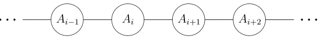
Consider a network of agents without cycles, where every agent has exactly M neigh-bors. Because of the same number of neighbors for each agent, the network looks the same way no matter which agent we place at the center. An example of such a network for M = 4 is given in Figure 1.
✣✢ ✤✜
✒✑ ✓✏ ✒✑ ✓✏
✒✑ ✓✏
[image:8.612.228.368.406.546.2]✒✑ ✓✏
Figure 1. An example of a network forM = 4.
There is one kind of information (for example, some particular technology) every agent can use to extract a one-time utility u. Time is discrete, t ∈ N. At t = 0 the agents
always knows who of his neighbors is informed; however, no one knows anything about his neighbors’ neighbors.
At each period starting from t = 1, the informed agents (sellers) decide on making offers to their uninformed neighbors (buyers). If made, the offer is a price at which the seller agrees to share the information with a buyer. The sellers who decide to wait with an offer can make it next period of time, if the neighbor is still uninformed. The sellers make the decision about the offers and set the prices separately for each of their uninformed neighbors. At the end of the period, the uninformed agents who have at least one offer can accept one of them, or wait.
The discount factor equalsδ ∈(0,1). All the agents are risk neutral. The agent’s utility att = 0 equals
U =
0, the agent is never informed;
δt(u−v) +W, the agent gets the information at period t,
where v is the price the agent pays for the information, and W is the total discounted revenue from selling the information to the neighbors. The agents maximize their expected utility.
2.2. The Strategies
At every period t agent α has history
Htα = ({sαtn}Mn=1,{(sαBtn , vtnαB)}Mn=1,{(sαStn , vtnαS,s˜αStn )}Mn=1,(sαt, mαt)), where
sα
tn — the time when neighbor n got informed;
sαBtn , vαBtn — the time when neighbor n made an offer, and the price offered;
sαStn , vtnαS,˜sαStn — the time of the offer to neighborn, the price and the time of acceptance, if any;
All the histories are consistent across the agents and across time.3 Denote H
t — the set of all possible histories at time t. The state of the world at time t is the set of all histories for all agents {Htα}α.
The buyer pure strategy is the decision to buy the information from one of the neighbors, or to wait (0 corresponds to waiting):
RαBt :Ht→ {0,1, . . . , M}.
The sellers pure strategy for each of the uninformed neighbors is the decision to wait (represented by∅, which is also played for the informed neighbors) or a price:
RtαS :Ht→ {R+,∅}M.
Denote the sets of pure strategies byRB
t and RSt respectively. We allow mixed strate-gies, i.e. some probability measuresµBt (·)∈∆(RBt ) and µSt(·)∈∆(RSt).
2.3. Equilibrium Definition
To find the equilibrium strategies we use Perfect Bayesian Equilibrium concept. This means that the agents play the best response to their histories in accordance with the beliefs, even if the histories are not achievable under the given equilibrium strategies. This equilibrium concept shares with the Perfect Bayesian Equilibrium the idea that every agent maximizes the expected utility in every state, given the system of beliefs consistent with all the other players’ strategies. Since there are infinitely many agents in the game, we can not directly apply the PBE concept, but need to generalize it in order to use it in our context. This generalization is similar in spirit to the local perfect equilibrium in Fudenberg, Levine, and Maskin [10] and is possible because at every period of time only a finite number of agents can influence the agent’s history.
Definition. A symmetric equilibrium of the game is a set of strategies {µBt (·), µS
t(·)}t≥0
such that no agent with any history (on or off the equilibrium path) can get extra payoff by deviating from his strategy given that all the other agents play the equilibrium strategies.
3By “consistent” we mean that the agents can not have contradictory histories. For example, if agent
The seller strategyµSt(·)}t≥0 is a product of identical distribution functions towards each
of the neighbors.
We consider symmetric equilibria, i.e. equilibria in which all the agents use the same strategies, and the strategies are symmetric with respect to different neighbors. The network does not contain cycles; therefore, the agent’s action towards one neighbor can not influence the decision of another neighbor, and based on this we assume that the agents act independently towards their different neighbors.
In the definition of an equilibrium the strategies depend on the history. The knowledge of the whole history is excessive and the decision might depend on a smaller number of parameters than the history contains. Also, we want to reduce the number of equilibria in the game by introducing the concept of equivalence between the equilibria.
The equivalence of two equilibria is understood in the following way. For the sellers, their expected revenue from selling the information to a particular uninformed neighbor does not change. What we change is when the offer is made. However, the offer itself (or a distribution of the offers) is the same and, although it is made at different period of time, the time of the acceptance does not change. For the buyers, if an informed neighbor does not make an offer, it means that the future offer is such that, made at the current period of time, it would not change the buyer decision on buying the information: the earlier offer does not change the buyer behavior. Consequently, the buyers in the equivalent equilibrium face the same distribution of the offers and the sellers make the offers with the same distribution as before. The expected utility of the agents is the same, although in the original equilibrium we need to take expectation with respect to the offers of the informed neighbors who wait with the decision to make their offers. The information diffuses in the same manner, and the fraction of the informed agents as well as the spacial structure of the informed/uninformed agents also stays the same.
The following proposition describes the necessary parameters and reduces the number of equilibria by introducing an equivalent equilibrium in which the sellers make their offers immediately after acquiring the information.
Proposition 1. For any equilibrium there exists an equivalent one, in which all the
function of offer prices Ft(v), and the buyer strategy is a function
Kt:{1,2, . . . , M} →R+,
which determines the reservation price for a given number of informed neighbors.4
We concentrate on the equilibria from proposition 1 at which the offers are made imme-diately, and the offers to different neighbors are independently drawn from distribution Ft(·). Denote
Vt = sup(suppFt(v))
— the highest possible price offered at time periodt. The buyers withlinformed neighbors accept the lowest offer if this offer does not exceed Kt(l).
The game has infinitely many agents and infinite horizon. Therefore, the equilibria may have the property of the Ponzi game, where the prices are not consistent with the utility the agents get from knowing the information. To exclude such equilibria from consideration, we use atransversality condition. We require that for any period of time t and for any l
Kt(l)≤u∗EAtl, (1)
where Atl stands for the random variable representing the discounted number of the uninformed agents who will get the information due to the transaction between the agent and the seller, if the buyer has exactlyl informed neighbors. This condition requires that the price does not exceed the expected discounted utility of all the agents who will get the information due to the transaction.
In equilibrium a buyer with all informed neighbors prefers to buy the information for any price not exceeding u. At the same time, buying the information for a price above u results in a negative payoff, therefore
Kt(M) = u. (2)
4We described here the strategies on the equilibrium path. The only deviation these strategies do not
take into account is the one when a neighbor gets the information and then does not make an offer. In
this case, we assume that the agent believes that the neighbor will make an offer next period of time,
and uses corresponding best response. This happens with probability zero, therefore we should not worry
A buyer immediately agrees on pricev ≤(1−δ)ubecause the loss in the expected utility from waiting is u−δu=u(1−δ). Therefore,
Kt(l)≥(1−δ)u ∀l ∈ {1,2, . . . , M −1}.
3. Linear Network
This section considers a special case of an infinite symmetric network without cycles — the infinite linear network (see Figure 2), where every agent has exactly two neighbors.
Ai−1
✣✢ ✤✜
Ai
✣✢ ✤✜
✣✢ ✤✜
Ai+1
✣✢ ✤✜
Ai+2
[image:13.612.133.447.322.363.2]q q q q q q
Figure 2. Infinite linear network.
3.1. General Results
The linear network, along with its plain structure, has the advantage of simple beliefs of the agents, which we can formulate using the following notation. Denote event “agent i is informed at time t” by At
i, and event “agent i is uninformed at time t” by Ati.
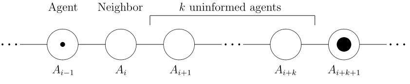
The following proposition describes the agent belief about the distance till the next informed agent. Although the fraction of the informed agents increases over time, this belief does not change as long as the agent himself and his neighbor stay uninformed.
Proposition 2. Suppose that all the agents in the linear network act independently
and use the same (even non-equilibrium) strategies. Then for any uninformed agent with
an uninformed neighbor his belief that there are exactly k other uninformed agents beyond
the uninformed neighbor has a geometric distribution with parameter p:
P(Ati−1Ati. . . Ati+kAt
i+k+1|Ati−1Ati) =p(1−p)k. (3)
q q q
Agent
Ai−1
✣✢ ✤✜
t
Neighbor
Ai
✣✢ ✤✜
✣✢ ✤✜
Ai+1
q q q
Ai+k
✣✢ ✤✜
⑦ ✣✢ ✤✜
Ai+k+1
q q q
[image:14.612.87.508.105.192.2]k uninformed agents
Figure 3. Illustration for Proposition 2.
necessary is that the strategies are the same (mixed or pure) for all the agents. Then Agent Ai−1 believes that the probability of k agents Ai+1, Ai+2, . . . , Ai+k to be uninformed and agents Ai+k+1 to be informed (this agent is marked with a black circle) equals p(1−p)k.
Probability that the next k agents are uninformed
P(Ati−1Ati. . . Ati+k|Ati−1Ati) =
∞ X
l=0
P(Ati−1Ati. . . Ati+kAti+k+l|Ati−1Ati)
=
∞ X
l=0
p(1−p)k+l= (1−p)k.
This result of Proposition 2 holds because of the following reasoning. First, the belief is calculated conditionally on the fact that the agent himself and his neighbor are unin-formed. In particular, Agent Ai−1 does not know anything about agents Al for l ≥ 1. Second, the initial distribution of the number of uninformed agents preceding the first informed one is geometric with parameter p because at the beginning everyone learns the information independently. And finally, the geometric distribution has the property similar to the constant hazard rate of the exponential distribution: the distribution of the difference of a geometrically distributed random variable and a constant (which models the diffusion of the information towards the agent) is the same as the distribution of the random variable if the difference is non-negative.
Suppose that the strategies are such that an uninformed agent with one offer always buys the information, i.e. Kt(1) ≥ Vt. Then the probability of acquiring the infor-mation by an uninformed neighbor of an uninformed agent equals p. (The product of P(Ati−1AtiAti+1|Ati−1Ati) = p and the probability that the information will be transferred, which equals one.) In other words,
P{Ati−1, Ait, Ati+1|Ati−1, Ati}=P{Ati−1, Ati, At
Consider a pure strategy equilibrium. In this equilibrium all the informed agents offer the information for the same price Vt at time t. The following proposition characterizes all such equilibria that satisfy the transversality condition.
Proposition 3. For any p ∈ (0,1) there exists at most one pure strategy equilibrium satisfying the transversality condition; for this equilibrium
Kt(1) =Vt= u
1−δ(1−p)2.
As the buyers and sellers use the same strategy every period of time in this pure strategy equilibrium, the information always diffuses from an informed agent to his uninformed neighbor if this neighbor has only one offer. The range for the initial parameter p when pure equilibria exists will be found in the next subsection.
3.2. Stationary Equilibria
Proposition 3 showed that in all pure strategy equilibria the strategies do not depend on time. Such equilibria, in which the strategies do not depend on time, Ft(·) = F(·), Kt(1) = K, we will call stationary equilibria. Equation 4 shows that if an agent with one only offer always buys the information, then the probability of an uninformed agent’s uninformed neighbor becoming informed equals p. This argument allows us to guess that there might be other stationary equilibria except for pure strategy equilibria. In this subsection we characterize all such equilibria.
All the possible strategies of stationary equilibria can be characterized using the fol-lowing proposition.
Proposition 4. In any stationary equilibrium K(1) = V. For any p ∈ (0,1) there exists exactly one stationary equilibrium. All stationary equilibria satisfy the transversality
condition. The type of the equilibrium depends on p:
1. For p∈0,2δ+1−2√δ4δ+1i
F(v)≡Fp(v) =
0, v < Vp; 1, v ≥Vp,
and Vp = u
2. For p∈2δ+1−2δ√4δ+1, p∗
F(v)≡F1m(v) =
0, v <(1−p)Vm
1 ; 1
p −
(1−p)Vm
1
pv , (1−p)V m
1 ≤v ≤u;
1
p −
(1−p)Vm
1
pu , u < v < V1m;
1, v ≥V1m,
and V1m > u is uniquely determined by equation
u (1−p)Vm
1
+δ(1−p)− 1 1−p =
δ 1−δ(1−p)
u (1−p)Vm
1
−1−ln
u (1−p)Vm
1
(5)
and decreases with p.
3. For p∈[p∗,1)
F(v)≡F1m(v) =
0, v <(1−p)Vm
1 ; 1
p − Vm
1 (1−p)
pv , (1−p)V1m ≤v ≤V1m;
1, v > V1m,
and
V1m = u(1−δ)
(1−δ(1−p))(1−δ(1−p)2) +δ(1−p) ln(1−p) ∈(0,1) (6)
is a decreasing function of p for p≥p∗.
Constant p∗ is the unique solution of equation
p−(1−δ(1−p))(1−p)2+ (1−p) ln(1−p) = 0 (7)
from interval 2δ+1−2√δ4δ+1,1.
[image:16.612.73.523.101.556.2]Different strategies F(v) for all three types of stationary equilibria are depicted at Figure 4.
For a smallpstrategyF(v) is a degenerate distribution with the mass point atVp > u, for a medium pstrategy F(v) has both continuous part on [(1−p)Vm
1 , u] and mass point
at V1m > u, and for a high p strategy F(v) is an absolutely continuous distribution on [(1−p)Vm
2 , V2m], where V2m ≤u.
Strategy F(v) for stationary equilibria evolves in the following way as pincreases (see Figure 5). For small p strategy F(v) = Fp(v) is a degenerate distribution with a mass point atVp > u, and this mass point decreases withp. Afterp= 2δ+1−√4δ+1
2δ , an absolutely continuous segment on [(1−p)Vm
✲ ✻
v 1
u Vp Fp(v)
✲
r
✲ ✻
v 1
u V1m (1−p)Vm
1
F1m(v)
✲r
✲ ✻
v 1
V2m (1−p)Vm
2 u
[image:17.612.69.505.139.275.2]F2m(v)
Figure 4. Stationary equilibra strategies in the infinite linear network.
Left graph: pure strategy Fp(v); Center graph: strategy Fm
1 (v); Right
graph: strategyF2m(v).
0 2δ+1−2√δ4δ+1 p∗ 1
Fp(v) F1m(v) F2m(v)
Figure 5. Stationary Equilibria Regions.
p)Vm
1 decreases) and the mass pointV1m decreases touwith the mass atV1m decreasing to
zero. At p=p∗, the mass point disappears, and the absolutely continuous segment starts moving towards zero. The lower bound decreases to 0, and the upper bound decreases to u(1−δ). Distribution F(v) weakly converges to the degenerate distribution with mass point at 0.
For p ∈ (0, p∗) there exists a mass point at V > u. Because this mass point is above
the agent’s personal valuation of the information, there is a non-zero probability that the agent will get two offersV at the same time, and therefore will stay uninformed forever. Proposition 5. In the stationary equilibrium with p ∈ (0, p∗) probability that an uninformed agent with two uninformed neighbors will stay uninformed forever equals
p(1−F(u))2
[image:17.612.133.439.387.432.2]Probability that a randomly chosen agent will stay uninformed forever can be calculated as the sum of two probabilities: (1) the probability that the agent and his neighbors were initially uninformed multiplied by the probability that the agent will stay uninformed forever, and (2) the probability that the agent has two informed neighbors each of which offers price above u:
(1−p)3p(1−F(u))
2
2−p + (1−p)p
2(1
−F(u))2 = (1−p)p(1−F(u))
2
2−p .
Forp≥p∗ every agent in the network will get informed. This thresholdp∗ divides interval (0,1) into the areas of efficient and non-efficient equilibria. In order to achieve efficiency, the central planner does not need to give the information to everyone; it is enough to give the information randomly to a sufficient fraction of the population.
The equilibria of the game, in particular the stationary equilibria, might not be robust with respect to some modifications of the game. The question is what happens with the strategies if we consider the same game with a finite horizon instead of the infinite one. Take a sequence of equilibria in the games with the time limited by T. We want to investigate how close are the equilibria in such finite horizon games to the infinite horizon game equilibria, i.e. the limit of the equilibria of the games with finite horizons.
Proposition 6. For small enoughpthe equilibria for the finite horizon games converge
to the pure strategy stationary equilibrium for the infinite horizon game.
3.3. Equilibria with Unbounded Price
The transversality condition restricts the prices. In this subsection we construct an example with a family of strategies in which this condition is not satisfied. The prices offered exceed some level and increase to infinity with time. What the agents pay for the information is not justified by the utility of the agents who get the information due to the transaction; the current price is supported by the expectations of the higher prices in the future.
holds for any t:
u−Vt+δ(1−p)2Vt+1 = 0,
i.e. buying the information and offering it to the uninformed agent gives zero expected utility. After rearranging the terms, one can get
Vt+1−
u
1−δ(1−p)2 =
Vt− 1−δ(1u−p)2
δ(1−p)2 .
Taking into account that in the stationary pure strategy equilibrium price always equals ¯
V = u
1−δ(1−p)2, we get
Vt+1−V¯ =
Vt−V¯
δ(1−p)2. (8)
As δ(1−p)2 <1, difference V −V¯ grows exponentially if initial V
0 exceeds ¯V:
Vt= ¯V + (V0−V¯)
1 δ(1−p)2
t
.
The only additional requirement for V0 is that a seller does not deviate to offering u
at t = 0, i.e. V0(1−p) > u (if the prices increase, it will also be true for arbitrary t).
Therefore, for any
V0 >max
u 1−p,
u 1−δ(1−p)2
the equilibrium we get is a pure strategy equilibrium for which the transversality condition fails, and the prices increases to infinity with time.
4. Random Networks
The analysis of the fixed networks showed that some equilibria in such networks possess some properties, like the price does not converge to zero. In this section we want to consider random networks, and find the properties of equilibria in these random networks to compare them with the properties of equilibria of the fixed networks.
Suppose that every period of time the agents are randomly matched with exactly M other agents5, and the network formed does not contain cycles. It means that at every
5Random network is a controversial issue, although it is used in many models. In this paper we do not
discuss the question of existence of such networks (although we believe that it is possible to construct a
period of time a new M-network or a set of them is formed, and no past history can influences the agents’ current decisions. Therefore, the agents’ actions are independent across the time and neighbors.
As before, all the informed agents can simultaneously make their offers to their unin-formed neighbors, and the uninunin-formed agents decide to accept one of the available offers or to wait. As we deal with the random network, the informed agents make their offers to uninformed neighbors every period of time, and the offers made expire at the end of each period with the abortion of the connections.
At the beginning, every agent independently with probabilityplearns the information. The seller strategy is a distribution function of offers Ft(v). The buyer strategy is a threshold Kt — the maximal price at which he is ready to buy the information. As new network is randomly formed each period of time, Kt does not depend on the number of informed neighbors. We consider only symmetric equilibria, i.e. the agents use the same strategies.
As before, denote Vt = sup suppFt(·). Threshold Kt ≥ Vt because otherwise offer Vt > Kt will never be accepted. Distribution function Ft(·) is absolutely continuous because Kt ≥ Vt and the agents will try to avoid the competition from other agents at the mass points. Also, Kt ≤ Vt because otherwise the agents selling the information for price Vt< Kt will be able to increase their offer to Kt without decreasing the probability of the deal. Therefore, Kt coincides with Vt, and later in this section Vt will represent both constants.
FromKt=Vtfollows that an agent becomes informed once he has at least one informed neighbor. Denote the probability of being informed at the beginning of period t by pt, with p1 =p. Then
pt+1 =pt+ (1−pt)(1−(1−pt)M) = 1−(1−pt)M+1; 1−pt+1 = (1−pt)M+1,
and pt monotonically approaches 1.
neighbors can have any influence on each other in the future. In particular, the probability of being
Denote
gt= (1−pt)M−1(M + (1−pt)). (9) As pt monotonically approaches 1,gt monotonically approaches 0.
As before, by the transversality condition we understand that the price in the trans-actions does not exceed the discounted expected utility of all the agents who get the information due to this transaction. The following proposition completely characterizes equilibria satisfying the transversality condition.
Proposition 7. For any initial probability p∈(0,1)there is only one equilibrium that satisfies the transversality condition. In this equilibrium the seller strategy
Ft(v) = 1 pt −
1−pt pt
Vt v
M1
−1
; (10)
suppFt(·) = [Vt(1−pt)M−1, Vt]. (11)
The highest price possible at period t
Vt = V1
t
Y
i=2
1 δgi −
u(1−δ) t
X
i=2
t
Y
j=i 1 δgj
; (12)
V1 = u(1−δ) 1 +
∞ X
i=3
i−1
Y
j=2
δgi
!
<∞. (13)
The highest possible price Vt monotonically decreases to u(1−δ), and the expected price
EFtv converges to 0.
As we see,Vtis uniquely determined by constantsM,p,u, andδ. Ft(·) weakly converges to the degenerate distribution with the mass point at zero.
5. Conclusion
the price. In the case of many uninformed agents at the beginning, this belief leads to the price exceeding the personal valuation of the information.
Not all the agents might learn the information at the end if the price exceeds the personal valuation; it happens if the information is a scarce resource. The information diffuses to all the agents if the fraction of the initially informed agents is large enough. Therefore, if the government wants everyone to have the information, it does not need to give it to all the agents; it is enough to exceed some threshold, and after this the agents will successfully trade the information with each other.
The linear network considered in many papers does not constitute a representative example. It has the property which is particular only for such a network: the belief about the number of uninformed agents till the first informed one, conditional on the fact that the agent himself and his neighbor are uninformed, does not depend on time. Due to this there exists the stationary equilibrium where the strategies the agents use do not depend on time.
References
1. Bala, Venkatesh, and Sanjeev Goyal. 1998. “Learning from Neighbors.” Review of Economic Studies
65(3), pp. 595-621.
2. Banerjee, Abhijit V., and Kaivan D. Munshi. 2000. “Networks, Migration and Investment: Insiders
and Outsiders in Tirupur’s Production Cluster.” MIT Department of Economics Working Paper
Series No. 00-08.
3. Belli, Pedro. 1997. “The Comparative Advantage of Government: a Review.” World Bank Policy
Research Working Paper No. 1834.
4. Billingsley, Patrick. 1995. “Probability and Measure.” Edition 3. New York: John Wiley & Sons.
5. Boyd, Robert, and Peter J. Richerson. 2005. “Solving the Puzzle of Human Cooperation,” In:
“Evolution and Culture,” S. Levinson ed. MIT Press, Cambridge MA, pp. 105-132.
6. Chatterjee, Kalyan, and Susan H. Xu. 2004. “Technology Diffusion by Learning from Neighbors.”
Advances in Applied Probability 36(2), pp. 355-376.
7. Conley, Timothy G., and Christopher R. Udry. 2000. “Learning About a New Technology: Pineapple
in Ghana.” Economic Growth Center Discussion Paper No. 817. New Haven: Yale University.
8. Eshel, Ilan, Larry Samuelson, and Avner Shaked. 1998. “Altruists, Egoists, and Hooligans in a Local
Interaction Model.” American Economic Review 88(1), pp. 157-179.
9. Foster, Andrew D., and Mark R. Rosenzweig. 1995. “Learning by Doing and Learning from Others:
Human Capital and Technical Change in Agriculture.” Journal of Political Economy 103(6), pp.
1176-1209.
10. Fudenberg, Drew, David K. Levine, and Eric Maskin. 1994. “The Folk Theorem with Imperfect
Public Information.” Econometrica 62(5), pp. 997-1039.
11. von Hippel, Eric. 1988. “The Sources of Innovation.” New York: Oxford University Press, 218 p.
12. Muto, Shigeo. 1986. “An Information Good Market with Symmetric Externalities.” Econometrica
54(2), pp. 295-312.
13. Polanski, Arnold. 2007. “A Decentralized Model of Information Pricing in Networks.” Journal of
Appendix
Lemma 1. The differential equation
af′(x)x= 1−bf(x)
forb6= 0,a6= 0 has solution
f(x) = 1
b −Cx
−b/a. (14)
Proof of lemma 1.
The solution is verified by substituting formula (14) for f(x) into the original equation and
the fact that the first-order differential equation has only one undetermined constant.
Proof of proposition 1.
The neighbors are connected only through the agent, therefore the seller strategy can be
independent for each of his uninformed neighbors; if the offer is made, it follows some distribution
functionFt(v), which depends only on time.
Suppose that a buyer with exactlyl informed neighbors accepts offerv. Then accepting offer
v′< v increases the buyer’s expected payoff by v−v′ without changing his expectations of the
future resales. The expected utility of waiting with the lowest offerv′< v increases by less than
v−v′ because the best difference is v−v′ and the discount factor decreases it. Therefore, the
strategy of a buyer with linformed neighbors is to accept an offer either from interval [0, Kt(l))
or [0, Kt(l)] for someKt(l)≥0. The buyer is indifferent to accept offer Kt(l) or to wait.
If for a buyer there is no mass of offers atKt(l), then these two options (to buy immediately
and to wait) do not differ, and we can choose the closed interval. If there is a mass point,
then the sellers who create the mass point (Ft(·) has a mass point) would prefer to deviate to
Kt(l)−ǫ, which means that this is not an equilibrium and Kt(l) can not be a mass point of
offers. Therefore, we can always assume that a buyer with l neighbors accepts any offer not
exceedingKt(l).
To prove the existence of an equivalent equilibrium in which all the sellers make their offers
immediately, consider one informed agent A and his uninformed neighbor B. By waiting agent
A can observe only the fact that B gets the information from his other neighbor (what makes
impossible selling the information to B). Agent A makes such offervthat maximizes his expected
payoff.
Option 1. Agent B with non-zero probability may accept offer v earlier than agent A
normally makes it. Then agent A is strictly better off by making the offer earlier, and therefore
this is not an equilibrium to delay with making this offer.
Option 2. Agent B would not accept offer v earlier than agent A normally makes it. Then
by making offer v earlier Agent A does not change his own payoff and the rest of his strategy.
Suppose that Agent B has other lowest offer and making offer v earlier changes B’s behavior.
As B does not accept offer v (we excluded option 1) then the other offer he has is better, and
B knows it because A does not make an offer. Consequently, revealing v does not change B’s
decision to accept other offers. Therefore, making offerv earlier does not change anything and
making the offers as soon as possible is a new equivalent equilibrium.
Proof of proposition 2.
The proof has the following structure. First, we consider the following modification of the
game: agents Ai, Ai−1,. . . are always uninformed at the beginning (see Figure 3). Second, we
demonstrate that random variables ξ1 and ξ1 −ξt are independent for any t, where ξt is the
number of uninformed agents Ai+1, Ai+2,. . . , Ai+k till the first informed agentAi+k+1 at time
t. Third, we show that ξt conditional onξt≥0 has the same geometric distribution as ξ1. And
last, we return to the original game, and prove formula 3 from the Proposition.
Step 1. Defining the game and random variables.
Suppose that Ai, Ai−1,. . . are always uninformed at the beginning. Define random variable
ξt∈Z in the following way:
ξt= min{k:Ai+k+1 is informed at the beginning of periodt}.
Random variableξt∈Zstands for the first informed agent in the network.
Step 2. Independence of ξ1 and ξ1−ξt.
Consider agent l who acquires the information at periodt. Let ηlt be the number of periods
it takes for agentl to transfer the information to his left neighbor, if this neighbor has only one
offer. The agents act independently, therefore all random variables{ηlt}are independent of each
other andξ1. The agents use the same strategies, therefore{ηlt}l are identically distributed for
each t.
Letηlstands for the number of agents the information diffused to the left by timetif initially
independent of ξ1 for any l (but not from each other). As {ηlt}l are identically distributed for
each t,ηl are identically distribute for everyl. Denote this distribution byη.
Note that
P(ξ1 =m, ξ1−ξt=l) = P(ξ1=m, ηξ1 =l) =P(ξ1=m, ηm =l)
= P(ξ1=m)P(η =l);
P(ξ1−ξt=l) = X
m
P(ξ1=m, ξ1−ξt=l) = X
m
P(ξ1 =m)P(η=l) =P(η=l),
i.e. random variablesξ1 and ξ1−ξt are independent.
Step 3. Geometric distribution ofξt conditional on ξt≥0.
We want to prove
P{ξt=k|ξt≥0}=p(1−p)k, ∀t, k∈N. (15)
Note that this formula holds for t = 1 because the agents independently with probability p
get the information at the beginning.
P{ξt=k|ξt≥0} =
P l≥0
P(ξ1=k+l, ξ1−ξt=l)
P l≥0,k′≥0
P(ξ1 =k′+l, ξ1−ξt=l)
=
P l≥0
p(1−p)k+lP(ξ
1−ξt=l)
P l≥0,k′≥0
p(1−p)k′+l
P(ξ1−ξt=l)
=
(1−p)kP l≥0
p(1−p)lP(ξ1−ξt=l)
1
p P l≥0
p(1−p)lP(ξ
1−ξt=l)
=p(1−p)k,
i.e. formula 15 holds for any t.
Step 4. Proof of formula 3 from the Proposition.
Consider the original game. In this game, agentsAi−1, Ai, can get the information by time
t either at the beginning, fromAi−2, or from Ai+1. We considered the process from the right.
We can make the same analysis from the left, and consider corresponding random variableζt—
the distance from the right informed agent to Ai−1 in the hypothetical network where all the
agents Ai−1, Ai, . . . are uninformed at the beginning, Then ξt and ζt are independent, and for
any k≥0
P(Ati−1Ati. . . Ati+kA¯ti+k+1|Ati−1Ati) = P(ζt≥0, ξt=k|ζt≥0, ξt≥0) = P(ζt≥0, ξt=k)
P(ζt≥0, ξt≥0)
= = P(ξt=k)
P(ξt≥0)
=p(1−p)k.
Consider first t such that Vt ≤ u. Consider an agent who makes an offer at time t to his
uninformed neighbor. There is a non-zero probability that the neighbor has the same offer
Vt from his another neighbor, and will be choosing the best one. Then the agent will benefit
by decreasing his offer to Vt−ǫ: the probability of selling the information increases, and the
payment stays almost the same. Therefore,Vt> u for allt.
Suppose that there exists t such that Vt < Kt(1). The agent accepts offer Vt only if this is
the only offer, and another neighbor is uninformed. By increasing the offer to Kt(1) the seller
does not decrease the chance of the deal, but increases the payment. Therefore, Vt can not be
less thanKt(1).
At every period of time there is either no trade or all the agents with one informed neighbor
only buy the information.
Consider first t such that Vt = Kt(1), Vt+1 > Kt+1(1). Suppose that t > 1 (the proof with
slight modification works for t = 1, too.) The agents with one offer Vt+1 only at time period
t+ 1 wait with the purchase until some period τ > t+ 1 with Vt+1 ≤ Kτ(1), and there is no
trade in periodst+ 1, t+ 2, . . . , τ−1.
Any agent who buys the information at periodthas utility zero because the offer from other
neighbors will exceedu, and the seller has all the power. Therefore,
−Vt+u+δτ−t(1−p)2Vt+1 = 0. (16)
Suppose that some agent with one the only offer Vt at period t does not buy the information
immediately, but waits till periodt+ 1. If his neighbor still stays uninformed, then he paysVt
at periodt+ 1, and offers it to his uninformed neighbor at timet+ 2≤τ forVt+1. Then, using
equation 16, his utility
δ(1−p)(−Vt+u+δτ−t−1(1−p)Vt+1) = δ(1−p)(−Vt+u) +Vt−u
= (Vt−u)(1−δ(1−p))>0
because Vt > 0, which means that this is not an equilibrium. The intuition behind the fact
the the utility increases if the agent waits is the following: by waiting the agent decreases the
uncertainty about the possibility of reselling the information.
We have proved that for any periodt holds Vt =Kt(1). Equation 16 forτ =t+ 1 gives us
the the law of motion forVt:
Fixed point
V = u 1−δ(1−p)2. Therefore,
Vt−V =δ(1−p)2(Vt+1−V),
which means that this fixed point is unstable: if V1 6= V then Vt converges either to −∞ or
to +∞. The first option contradicts Vt ≥0, and the second one contradicts the transversality
condition (the price is limited by some constant).
Proof of proposition 4.
First, we want to show that V = K(1). We already know that K(2) = u. Distribution
function F(v) is continuous for v ≤ u because Kt(2) = u and a seller offering the mass point
price would better off by decreasing his offer by small ǫto avoid the tie.
Suppose that V 6= K(1). As V ≤ max(K(1), u), the following four options are possible:
V < K(1)≤u,K(1)< V ≤u,V < u≤K(1), andu≤V < K(1).
Options V < K(1) ≤ u and V < u ≤ K(1) can not be an equilibrium because F(v) is
continuous belowu, and a seller offering the information for priceV is better off by askingK(1)
and u correspondingly.
Consider option K(1) < V ≤ u. There is a non-zero probability of offers v ∈ [0, K(1)] and
v ∈ (K(1), u] because otherwise an agent with offer K(1) will not get be able to get a better
offer in the future. An offer from [0, K(1)] is always accepted, and an offer from (K(1), u] is
accepted if and only if there are two offers; in the case of one offer the agent always waits for
the second one. Because of the waiting the agents change their belief about event “the first
informed agent behind the uninformed neighbor got an offer aboveK(1),” which is impossible
in stationary equilibrium. Therefore,K(1)< V ≤u is not an equilibrium.
Consider optionu≤V < K(1). OffersV andK(1) have the same chance to be accepted (the
neighbor’s neighbor is uninformed and stays uninformed till the next round), butK(1) delivers
a higher payoff. Therefore, this is also not an equilibrium.
We have proved that either V = K(1) < u or u < V = K(1). Later in the proof we will
always use V instead ofK(1), The support ofF(v) belowu constitutes a connected set; if not,
an agent can increase his expected payoff by increasing the offer in the gap as the probability
There are 3 cases: F(u) = 0, F(u)∈(0,1), andF(u) = 1. If F(u)<1, then the distribution
of pricesF(v) has mass 1−F(u) atV > u. IfF(u)>0, then the expected payoff maximization
problem for v∈[0,min(u, V) gives
(1−p)v+pv(1−F(v))→max; (17)
1−pF(v)−pvf(v) = 0.
Applying Lemma 1,
F(v) = 1
p − C
v forv∈[pC,min(u, V)].
OfferpC is always accepted, and offerV is accepted only of there is the neighbor does not have
other offer. Both these prices are in the support ofF(·) and deliver the same expected payoff,
therefore pC= (1−p)V, and
F(v) = 1
p−
(1−p)V
pv forv∈[(1−p)V,min(u, V)].
Now we want to findF(v) for each of the three cases.
Case 1. F(u) = 0, pure strategy with mass 1 atV > u.
Denote this distribution function of offers byFp(v). In accordance with Proposition 3,V = u
1−δ(1−p)2. This equilibrium exists if and only if the agents do not want to offer priceu which is always accepted, i.e.
V(1−p)≥u;
p≤δ(1−p)2; (18)
Case 2. F(u)∈(0,1), some mass at V > uand a continuous part on [(1−p)V, u].
Denote this distribution function of offers byFm
1 (v).
An agent with offerV and one uninformed neighbor is indifferent between accepting the offer
and waiting for another one. The expected payoff from buying the information immediately
equals
If the agent waits for another offer, he gets the information if and only if his another neighbor
offers the information for a price v≤u. The expected payoff from waiting is
E
X
t≥1
δtp(1−p)t−1(u−v)I{v≤u}
=
pδ
1−δ(1−p)
F(u)u− u Z
(1−p)V
v d F(v)
= (1−p)V δ 1−δ(1−p)
u
(1−p)V −1− u Z
(1−p)V d v
v
= (1−p)V δ 1−δ(1−p)
u
(1−p)V −1−ln
u
(1−p)V
.
Equating the expected payoff of from buying the information immediately (formula 19) and
waiting, one gets equation 5:
u
(1−p)V +δ(1−p)−
1 1−p =
δ
1−δ(1−p)
u
(1−p)V −1−ln
u
(1−p)V
. (20)
The condition for the existence of such equilibriumF(u)∈(0,1) is equivalent tox≡ (1−up)V ∈
1,1−1p. Rewriting equation 20 usingx gives
x− δ
1−δ(1−p)(x−1−lnx) = 1
1−p−δ(1−p). (21)
Denote the left-hand side of equation 21 by h(x, δ, p). For anyx∈h1,1−1pithe derivative
∂h(x, δ, p)
∂x = 1−
δ(1−1/x)
1−δ(1−p) ≥1−
δ(1−(1−p)) 1−δ(1−p) =
1−δ
1−δ(1−p) >0;
Therefore, there exists x∈1,1−1psatisfying equation 21 if and only if
h(1, δ, p)< 1
1−p −δ(1−p)< h
1 1−p, δ, p
; (22)
1< 1
1−p −δ(1−p)<
1 1−p −
δ
1−δ(1−p)
p
1−p−ln
1 1−p
.
Therefore, this equilibrium exists if and only if the following two inequalities hold:
p > δ(1−p)2; (23)
−(1−δ(1−p))(1−p)2+p+ (1−p) ln(1−p)<0. (24)
Denote this distribution function of offers by Fm
2 (v). A buyer is indifferent between buying
at the maximal priceV (formula 19) and waiting:
−V +u+δ(1−p)2V = X
t≥1
δtp(1−p)t−1
Z
(u−v)dF(v) = (1−p)V δ 1−δ(1−p)
V Z
(1−p)V u−v
v2 dv
= (1−p)V δ 1−δ(1−p)
−u
V + u
(1−p)V
+ ln(1−p)
= pδu
1−δ(1−p)+
(1−p)V δln(1−p) 1−δ(1−p) ;
V = u(1−δ)
(1−δ(1−p))(1−δ(1−p)2) +δ(1−p) ln(1−p). This equilibrium exists if and only ifV ≤u, or
−(1−δ(1−p))(1−p)2+p+ (1−p) ln(1−p)≥0. (25)
We want to show that for anyδ ∈(0,1) interval (0,1) is divided into three parts by p′∈(0,1)
and p′′ ∈ (p′,1). On (0, p′] inequality 18 holds (Case 1), on (p′, p′′) inequalities 23 and 24 hold
(Case 2), and on [p′′,1) inequality 25 holds (Case 3).
Inequality 18 holds on (0, p′] and inequality 23 holds on (p′,1), where
p′ = 2δ+ 1−
√
4δ+ 1
2δ .
Denote left-hand side of inequalities 24 and 25 as g(p, δ). The second derivative
∂2
∂p2
g(p, δ)
1−p
= ∂
∂p
(1−δ(1−p))−δ(1−p) + 1 1−p +
p
(1−p)2 − 1 1−p
= 2δ+ 1
(1−p)2 + 2
p
(1−p)3 >0,
therefore g1(p,δ−p) either increases or first decreases and then increases. Asg(0, δ)<0 andg(0, δ)>
0, equation g(p, δ) = 0 has exactly one solution p′′ ∈ (0,1), and on (0, p′′) inequality 24 holds,
and on [p′′,1) inequality 25 holds. The only fact we have to prove is thatp′′> p′. To do this, it
is enough to show that there exists p satisfying both inequalities in 22.
We know that h(1, δ, p′) < h1−1p′, δ, p′
, h(1, δ, p) = 1, h(1, δ, p′) = 1−1p′ −δ(1−p′), and
functionh(x, δ,p˜) is continuous in all arguments. The middle part of 22 increases withpbecause
1
1−p −δ(1−p) = (1−δ) +p(1 +δ) +p
2+p3+. . . .
Therefore, in some neighborhood of p′ for p > p′ both inequalities in 22 hold, and therefore
ValueVm
2 decreases withp because p > δ(1−p)2 and therefore
d dp
u(1−δ)
δVm
2
= 1−δ(1−p)2+ 2(1−p)(1−δ(1−p))−1−ln(1−p)
≥ 1−p−1−ln(1−p)≥0.
ValueV1m decreases withp because p > δ(1−p)2 and therefore
d dp
u(1−δ)
δV2m
= 1−δ(1−p)2+ 2(1−p)(1−δ(1−p))−1−ln(1−p)
≥ 1−p−1−ln(1−p)≥0.
Proof of proposition 5.
The agent will get two offers simultaneously only if the informed agents on the opposite sides
are located on the same distance. Therefore, the probability of staying uninformed forever equals
X
t≥0
((1−p)tp)2(1−F(u))2 =p2(1−F(u))2 1
1−(1−p)2 =
p(1−F(u))2
2−p .
Proof of proposition 6.
We will denote all the strategies in the game with horizonT by upper indexT. We are looking
for the finite horizon equilibria at which the agents with one informed neighbor only always buy
the information, i.e. VT
t =KtT(1).
At the last period K(1) = u and therefore FT
T(u) = 1,. The seller’s problem is the same as
problem 17, which means that the solution is also the same:
FTT(v) = 1
p
1−u(1−p)
v
, v∈[(1−p)u, u].
The expected payoff of the agent who gets only one offer is
π≡ u Z
(1−p)u
(u−v)dFTT(v)≤
u Z
(1−p)u
(u−(1−p)u)dFTT(v) =pu.
Suppose that for anyt < T distribution function FtT(v) has mass 1 atV =KtT(1)> uand does
not have the continuous part below u. Then to make the buyer indifferent between buying and
waiting till the last period the following equation should hold:
−VtT +u+δ(1−p)2VtT+1 = δT−t(1−p)T−t−1pπ (26)
Note that
Note thatVT
T < 1−δ(1u−p)2. By induction,
VtT =−δT−t(1−p)T−t−1pπ+u+δ(1−p)2VtT+1< u+ δ(1−p) 2u
1−δ(1−p)2 =
u
1−δ(1−p)2.
Note thatVTT−1> VTT. By induction,VtT−1 > VtT because
VtT−1 = −δT−(t−1)(1−p)T−(t−1)−1pπ+u+δ(1−p)2VtT
> −δT−t(1−p)T−t−1pπ+u+δ(1−p)2VtT+1 =VtT.
No seller will deviate fromVtT because the expected payoff fromVtT is greater than the expected
payoff from u:
(1−p)VtT ≥(1−p)VTT−1>(1−p)(u(1 +δ(1−p)2)−pu)> u,
where the last inequality holds for small enoughp.
Finally, for any t values VtT converge as T increases because VtT are limited, increase, and
VtT+1+1 =VT
t . Denote Vt= lim T→∞V
T
t . Then
V −VtT =δ(1−p)2(V −VtT+1) +δT−t(1−p)T−t−1pπ;
V −Vt=δ(1−p)2(V −Vt+1).
Vt are limited, and have the same law of motion as Vt for the pure strategy equilibrium,
therefore Vt= 1−δ(1u−p)2 for anyt.
Proof of proposition 7.
The structure of the proof is the following. First, we show that Ft(·) does not have mass
points and has a connected support for any t. Second, we prove that
Ft(v) =
1
pt − Ctv−
1
M−1. (27)
and find formula for the support (formulas 10 and 11). Third, we prove the law of motion for
Vt:
1
δ(Vt−1−u) =Vtgt−u. (28)
Forth, based on the law of motion forVt we establish formulas 12 and 13 for Vt. And last, we
show monotonicity and convergence of Vt and convergence ofEFtv.
No offer aboveVtwill be accepted, thereforeFt(Vt) = 1. The distribution function Ft(·) does
not have mass points because otherwise a seller would prefer to decrease his offer from these
mass points by some small ǫ.
The support supp(Ft(·)) is connected because by increasing the offer in the gap, a seller will
increase his expected payoff as the acceptance probability of the offer stays the same, and the
price increases.
Step 2. The proof of formulas 10 and 11 forFt(·) and for its support.
The expected payoff from one uninformed neighbor is equal to
πt(v) = vP{v≤other offers}
= v
M−1
Y
i=1
(P{v≤offer from neighbor i}+P{no offer from neighbori})
= v
M−1
Y
i=1
((1−Ft(v))pt+ (1−pt)) = (1−ptFt(v))M−1v.
All the points in the support of Ft(·) should deliver the same utility π, we have
π′t(v)≡(1−ptFt(v))M−1−ptft(v)v(1−ptFt(v))M−2(M−1) = 0;
ptft(v)v(M−1) = 1−ptFt(v).
Applying Lemma 1,
Ft(v) =
1
pt −Ctv
− 1
M−1
for some constantCt>0 (formula 27).
One can verify that
Vt≡sup suppFt(·) =
ptCt
1−pt M−1
,
thereforeCt= 1−ptptV
1
M−1
t and we have proved formula 10 forFt(·) and formula 11 for the support
of Ft(·).
Step 3. Law of motion for Vt (formula 28).
LetUi
t be the expected payoff of an informed agent at the beginning of periodt, and let Utu
be the expected payoff of an uninformed agent at the beginning of periodt. Then
Uti = M(1−pt)πt+δUti+1 =
∞
X
i=t
δi−tM(1−pi)πi; (29)
whereEvtstands for the expected price an agent pays for acquiring the information at periodt,
conditional on the fact that there is at least one offer.
In an equilibrium the buyer with the highest possible offerVt is indifferent between accepting
the offer and waiting, therefore
u−Vt+δUti+1 =δUtu+1. (31)
Substituting expressions forUti (formula 29) andUtu (formula 30) into 31 one can get
1
δ(Vt−1−u) = M(1−pt) ˜Vt+δU i t+1
−(u−Evt+δUti+1)(1−(1−pt)M)−δUtu+1(1−pt)M
= (Vt−u)(1−pt)M +M(1−pt)MVt+ (Evt−u)(1−(1−pt)M)
= (M + 1)Vt(1−pt)M +Evt(1−(1−pt)M)−u. (32)
In order to simplify expression 32, we need formula for Evt.
The average minimal price from lindependent offersv, v2, . . . , vl is equal to
EFltv≡
Z
v dP(min(v1, . . . , vl)≤v) = Z
vd1−(1−P(v1 ≤v))l
=
Z
vd 1−
ht(v)−
1
pt −1
l!
=
Z
ht(v)l M−1
ht(v)−
1
pt
+ 1
l−1
dv, (33)
whereht(v) = 1−ptpt Vvt
1
M−1
for simplicity of notation. Note that
M X
l=1
lxl−1CMl plt(1−pt)M−l = M pt M−1
X
l=0
CMl −1xlplt(1−pt)(M−1)−l
= M pt(px+ 1−pt)M−1 (34)
Equation 34 forx=ht(v)−p1t + 1 gives
M X
l=1
l
ht(v)−
1
pt
+ 1
l−1
Combining 33 and 35 and swapping the integral and the sum, one can get
M X
l=1
CMl plt(1−pt)M−lEFltv =
Vt
Z
Vt(1−pt)M−1
M
M−1(ht(v)pt)
Mdv
=
Vt
Z
Vt(1−pt)M−1
M
M−1 (1−pt)
Vt
v
1
M−1
!M
dv
= Vt
1
Z
(1−pt)M−1
M
M−1(1−pt)
Mv− 1
M−1−1dv. (36)
Taking into account the fact that the probability of exactly l informed neighbors is equal to
CMl plt(1−pt)M−l and applying equation 36, we have
Evt(1−(1−pt)M) = M X
l=1
CMl plt(1−pt)M−lEFltv
= Vt
1
Z
(1−pt)M−1
M(1−pt)M
M−1 v
− 1
M−1−1dv
= −VtM(1−pt)Mv−
1
M−1
1
(1−pt)M−1
=VtM pt(1−pt)M−1. (37)
Substituting Evt(1−(1−pt)M) (formula 37) into formula 32 and taking definition for gt
(formula 9), we have the law of motion for Vt (formula 28).
Stage 4. Finding expression forVt(formulas 12 and 13).
Rearranging terms in formula 28, one can get
Vt= Vt−1
δgt −
u(1−δ)
δgt
. (38)
Formula 38 fort= 2 corresponds to the expression for Vt (formula 12). Using formula 38 again,
Vt+1 =
V1
t Q i=2
1
δgi −u(1−δ)
t P i=2
t Q j=i
1
δgj
δgt+1 −
u(1−δ)
δgt+1
= V1
t+1
Y
i=2 1
δgi −u(1−δ) t X
i=2
t+1
Y
j=i
1
δgj −
u(1−δ)
δgt+1
= V1
t+1
Y
i=2 1
δgi −
u(1−δ)
t+1
X
i=2
t+1
Y
j=i
1
which by induction proves formula 12 for any t >2. Now we want to prove formula 13 forV1.
Expressing V1 through Vt using formula 12 , we get
V1 =
Vt+u(1−δ) t X
i=2
t Y
j=i
1 δgj t Y i=2 δgi = Vt t Y i=2
δgi+u(1−δ)
1 +
t X
i=3
i−1
Y j=2 δgj
. (39)
Values Vt are limited by some constant because of the transversality condition, therefore
lim
t→∞Vt
t Y
i=2
δgi = 0
as limt→∞gt≡limt→∞(1−pt)M−1(M+ 1−pt) = 0. (Probabilitiesptconverge to 1.) Therefore,
taking limits both parts of 39 fort→ ∞, one gets formula 13 forV1.
To proveV1 <∞ notice that as values gt= (1−pt)M−1(M+ (1−pt)) converge to 0, for any
ǫ∈(0,1) there exists t0 such thatgt< ǫfor anyt > t0. Therefore,
V1
u(1−δ) −
1 +
t0
X
i=3
i−1
Y j=2 δgj = ∞ X
i=t0+1
i−1
Y
j=2
δgj < t0 Y j=2 δgj ∞ X
i=t0
ǫi−t0
<∞.
Step 5. Properties ofVt and EFtv.
Find expression for Vt in terms ofptand gt:
Vt = V1
t Y
i=2 1
δgi −
u(1−δ)
t X
i=2
t Y
j=i
1
δgj
= u(1−δ)
1 +
∞
X
i=3
i−1
Y j=2 δgj t Y i=2 1
δgi −
u(1−δ)
t X
i=2
t Y
j=i
1
δgi
= u(1−δ)
1 +
∞
X
i=t+2
i−1
Y
j=t+1
δgj
.
Values gtdecrease with time to zero. Therefore,
∞
X
i=t+2
i−1
Y
j=t+1
δgj <
∞
X
i=t+2
i−1
Y
j=t+1
δgj−1 =
∞
X
i=(t−1)+2
i−1
Y
j=(t−1)+1
δgj,
and Vt decreases with t. Also, if gj < g for anyj > t, then
∞
X
i=t+2
i−1
Y
j=t+1
δgj ≤
∞
X
i=t+2
(δg)i−(t+1) = δg 1−δg,