Inventory Model for Decaying Items with Multivariate
Demand and Variable Holding Cost under the Facility of
Trade-Credit
Anupam Swami
Assistant Professor Govt. P.G. College Sambhal, U.P.Sarla Pareek
Professor and HOD Banasthali UniversityJaipur, RAJ.
S.R. Singh,
Ph.D. Associate ProfessorCCS University Meerut, U.P.
Ajay Singh
Yadav,
Ph.D. Assistant ProfessorSRM University NCR Campus, GZB
ABSTRACT
In this study, an inventory model for deteriorating items with multivariate demand and variable holding cost is developed. The facility of allowable delay in payment is also taken into consideration. During this period retailer can use the ensued money from sales of the supplied goods to earn interest. Demand rate is a function of on hand inventory and selling price of the item and it is considered that the stock affects the demand rate up to an assured time. Therefore, retailer will order more quantity to stimulate demand rate and to earn more money. Different cases of allowable delay in payment are discussed. The objective of this study is to maximize the retailer’s total profit per unit time. The results are illustrated with some numerical examples and sensitivity analysis for each case is also carried out.
Keywords
Inventory Model, Sensitivity Analysis, and consumption rate
1.
INTRODUCTION
The classical inventory models consider the demand rate to be either constant or time-dependent but independent of the available stock status. However, in many practical situations customers’ purchasing manners may be affected by factors such as selling price, on hand inventory and so on. As deliberated by Levin et al. (1972) and Silver and Peterson (1985), sales at the retail point tend to be proportional to inventory displayed and a large piles of goods exhibited in a supermarket will escort the purchasers to buy more. Many marketing researchers and practitioners have paying attention to investigate the modelling aspects of this occurrence. Gupta and Vrat (1986) first designed a model for consumption environment to minimize the cost with the assumption that demand rate is a function of the initial stock level. Mandal and Phaujdar (1989), Datta and Pal (1990), Padmanabhan and Vrat (1995) further developed inventory models under stock-dependent consumption rate with some different assumptions. Since a firm may use a pricing strategy to stimulate demand for its seasonal goods, the inventory problems with selling price and stock dependent demand cannot be disregarded. Urban and Baker (1997) investigated a deterministic inventory problem in with multivariate demand rate. Datta and Paul (2001) analyzed an inventory system where the consumption rate of the goods is affected by both displayed stock level and selling price. You (2005) investigated an inventory model by considering price and time dependent demand rate. Some inspiring research articles associated to this research environment are, You and Hsieh (2007), Chang et al. (2010), Lee and Dye (2012).
In today’s business communications, it is more and more frequent to see that the supplier allows the retailer a fixed time (trade-credit) period. This provides an advantage to the retailer, as he/she does not has to pay the supplier immediately after receiving the items; in contrast during the delay period an interest can be earned by the retailer on the accumulated revenue. On the other hand, the strategy of allowing a permissible delay period is also beneficial for the supplier as it attracts new retailers/purchasers who consider this policy to be a type of purchasing cost reduction. Based on this phenomenon, Goyal (1985) analyzed the effect of trade credit on the optimal inventory policy. Later on, Aggarwal and Jaggi (1995) extended Goyal (1985) model with an exponential deterioration rate under the policy of allowable delay in payments. Jamal et al. (1997), Chang and Dye (2001) put forwarded inventory models with trade-credit policy by considering shortages. Teng (2002) proposed an inventory model by estimating the difference between unit selling price and unit cost and recognized an easy analytical closed-form solution to the problem. Sana and Chaudhuri (2008) analyzed optimal trade-credit policies when a price discount is offered. Khanra et al. (2011) proposed an EOQ (Economic Order Quantity) model for a deteriorating item having time dependent demand rate when delay in payment is permitted. Teng et al. (2012) deliberated an inventory model with non-decreasing demand and trade-credit financing.
The above mentioned literature reveals that inventory models for decaying items under the condition of allowable delay in payment with variable holding cost, stock and price dependent demand rate, while the on hand inventory affects the demand rate up to a assured period are not discussed so far. Therefore, in this study, an inventory model for deteriorating items with multivariate rate is developed. It is assumed that a trade credit period is offered by the supplier to the retailer. The time dependent holding cost is also taken into consideration. Three cases are discussed according to the situation of the delay period. To validate the concept of this study numerical examples are provided and sensitivity analysis for different cases is also discussed. The concavity of the profit function in each case is disclosed graphically.
2.
NOTATIONS AND ASSUMPTIONS
The following notation is used throughout the paper:
( )
I t
The inventory level at any timet
,t
0
T
Cycle length (time units)
Deterioration rate of on hand inventory during cycle time1
T
Time up to which demand is affected by on hand stocke
I
Interest earned (/$/cycle)c
I
Interest charges per $ investment in inventoryper cycle
M
The trade credit period length per cyclep
Unit selling price per item ($)h
t
Holding cost per unit per unit time ($)p
C
Purchasing cost per unit ($)d
C
Purchasing cost per unit ($)A
Ordering cost for placing an order ($/order)3.
ASSUMPTIONS
In developing the mathematical model, the following assumptions are made:
1. The demand rate,
D t
( )
is a function of stock and price and is defineD t
( )
a
bI t
( )
cp
,
where a is positive constant, b is the stock-dependent consumption rate parameter,0 b 1,
0
c
is the selling price dependent factor and I(t) is the inventory level at time t.2. The inventory system involves only one type of perishable item and the planning horizon is infinite.
3. The replenishment rate is infinite.
4. Holding cost per unit per unit time is
h
t
where0, 0
1
h
.5. The deteriorating rate,
(0
1)
, is constant and there is no replacement or repair of deteriorated units during the period under consideration.4.
MODEL FORMULATIONS
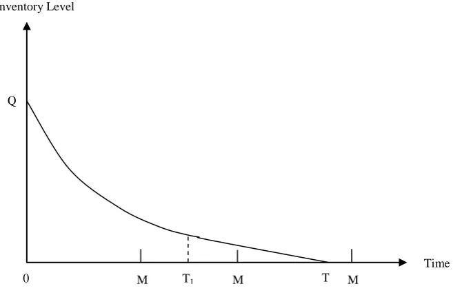
[image:2.595.142.484.376.590.2]Here, the replenishment policy of a deteriorating item with variable demand rate is considered. The objective of the inventory system is to determine the optimal ordering quantity and the length of ordering cycle. The behavior of the inventory system at any time t is depicted in Figure 1. There may arise three cases according to the position of the delay period M as shown in Figure 1.
Figure 1: The graphical representation of inventory system
Replenishment is made at time
t
0
and the order size is Q. During the period[0,
T
1]
the available stock and selling price of the item both affect the demand rate after that during the period[
T T
1, ]
only selling price influences the demand rate. The inventory level during the period[0, ]
T
decreasesdue to the combined effect of the demand rate and deterioration of the item and ultimately falls to zero at
t
T
. Hence, the differential equations representing the inventory status during the period[0, ]
T
are given by
'
1
( )
( )
( )
I t
I t
a
bI t
cp
0≤t≤T1 (1)
'
2
( )
( )
I
t
I t
a
cp
T1≤t≤T (2)With boundary conditions I1(0)=Q, I2(T)=0. Solving eq. (1) and (2) we get
T1 T
Inventory Level
Time Q
1
( )
b t
a
cp
a
cp
I t
Q
e
b
b
(3)
2
( )
1
T t
a
cp
I t
e
(4)Since inventory level is continuous at t=T1, so we have I1(T1)=I2(T1)
1
1
11
1T T b T b T
a
cp
a
cp
Q
e
e
e
b
(5)Now, ordering cost per unit time is OC and is given by
A
OC
T
(6)Purchasing cost per unit time is PC and is given by
p
C Q
PC
T
(7)Inventory carrying cost per unit time is HC and is given by
1 2 1 1 2 01
( )
( )
T T THC
h
t I t dt
h
t I
t dt
T
1 1 2 1 1 1 2 2 2 1 2 21
2
2
b T T Ta cp
h
h
T
b a cp
T
HC
Q
e
hT
T
b
b
b
b
b
b
a cp
h
T
h
T
a cp
T
e
hT
(8)Deterioration cost per unit time is DC and is given by
1 2 1 1 2 0
( )
( )
T T d TC
DC
I t dt
I
t dt
T
1 1 1 11
1
1
b T T Td
e
a
cp
a
cp T
a
cp
C
DC
Q
e
T
T
T
b
b
b
(9)Sales revenue per unit time is SR and is given by
1 1 1 0( )
T T TSR
p
a bI t
cp dt
a cp dt
1 11
e
b Ta cp
a cp T
SR
p
a cp T
b
Q
b
b
b
(10)Now, according to the position of delay period M there arise three cases:
Case (1) M ≤ T1 < T Case (2) T1
≤ M < T Case (3) M ≥ T
We shall discuss these three cases one by one.
Case (1): M ≤ T1 < T
During the credit period the buyer can use the sale revenue to earn an interest and can collect more capital. So, interest earned per unit time is IE1 and is given by
1 1 0( )
M epI
IE
a
bI t
cp tdt
T
2
1 2 2
1
1
2
b M
e
a
cp M
a
cp
pI
M
IE
b Q
e
T
b
b
b
b
b
(11)After, the credit period the buyer/retailer has to pay the interest for the goods still in stock with annual rate
I
c.
Therefore, interest charged per unit time is IC1 and is given by
1
1
1 1
( )
2( )
T T
p c
M T
C I
IC
I t dt
I
t dt
T
1 11 1 1
1
b M b T T T
p c
e
e
e
C I
a cp
a cp
a cp
IC
Q
T
M
T T
T
b
b
b
. (12)
The total profit per unit time for this case is AP1 and is given by
1
,
1 1AP T p
SR
IE
OC
PC
HC
DC
IC
(13)The objective of this study is to maximize the total profit per unit time AP1(T,p). The necessary conditions for maximizing the profit are
1
,
0
AP T p
T
(14)
1 ,
0
AP T p p
(15)
From equation (14) and (15) with the help of software Mathematica-8.0, we can determine the optimum values of T* and p* simultaneously and optimal order size (Q*) can be observed from (5). Also, the optimal value AP1(T
*
, p*) of the average profit can be determined by (13) provided they satisfy the sufficiency conditions that are given as follows:
2
2 2 2 2 2
1 1 1 1 1
2 2 2 2
( , )
( , )
( , )
( , )
( , )
0,
0
0
AP T p
AP T p
AP T p
AP T p
AP T p
and
T p
T
p
T
p
(16)Case (2): T1 ≤ M ≤ T
In this case, interest earned per unit time is IE2 and is given by
1 1
1
2 1 1 1
0 0
( )
( )
T T M
e
T
pI
IE
a
bI t
cp tdt
M
T
a
bI t
cp dt
a
cp tdt
T
1 1 1 2 2 2 1 1 1 2 2 1 11
2
2
1
b T b T e b Te
a
cp
M
T
a
cp T
a
cp
pI
T e
IE
b Q
T
b
b
b
b
a
cp T
b
a
cp
M
T
Q
e
b
b
b
.(17)For this case, interest charged per unit time is IC2 and is given by
2 2 1 ( ) T M Tp c p c
M
e
C I a cp C I
IC I t dt T M
T T
(18)The total profit per unit time for this case is AP2 and is given by
2
,
2 2AP T p
SR
IE
OC
PC
HC
DC
IC
(19)Again, the objective of this study is to determine the optimal values of T and p, when T1 < M ≤ T, in order to maximize the total profit per unit time AP2(T, p). The necessary conditions for maximizing the profit are
2
,
0
AP T p
T
2 ,
0
AP T p
p
(21)
From equation (20) and (21) with the help of software Mathematica-8.0, we can determine the optimum values of T* and p* simultaneously and optimal order size (Q*) can be
observed from (5). Also, the optimal value AP2(T*, p*) of the average profit can be determined by (19) provided they satisfy the sufficiency conditions that are given as follows
2
2 2 2 2 2
2 2 2 2 2
2 2 2 2
( , )
( , )
( , )
( , )
( , )
0,
0
0
AP T p
AP T p
AP T p
AP T p
AP T p
and
T p
T
p
T
p
(22)Case (3): T < M
In this case, interest earned per unit time is IE3 and is given by
1 1
1 1
3 1 1 1
0 0
( )
( )
T T T T
e
T T
pI
IE
a
bI t
cp tdt
M
T
a
bI t
cp dt
a
cp tdt
M
T
a
cp dt
T
1 1 1 2 2 2 1 1 1 3 2 1 1 11
2
2
1
b T b T e b Te
a
cp T
T
a
cp T
a
cp
pI
T e
IE
b Q
T
b
b
b
b
a
cp T
b
a
cp
M
T
Q
e
M
T
a
cp T
T
b
b
b
.(23)Interest charged per unit time is IC3 and is given by
3
0
IC
(24)The total profit per unit time for this case is AP3 and is given by
3
( , )
3 3AP T p
SR IE
OC PC HC DC IC
(25) The purpose of this study is to determine the optimal values of T and p, when M > T, in order to maximize the total profit per unit time AP3(T, p). The necessary conditions for maximizing the profit are
3
,
0
AP T p
T
(26)
3 ,
0
AP T p p
(27)
From equation (26) and (27) with the help of software Mathematica-8.0, we can determine the optimum values of T* and p* simultaneously and optimal order size (Q*) can be observed from (5).
Also, the optimal value AP3(T *
, p*) of the average profit can be determined by (25) provided they satisfy the sufficiency conditions that are given as follows:
2
2 2 2 2 2
3 3 3 3 3
2 2 2 2
( , )
( , )
( , )
( , )
( , )
0,
0
0
AP T p
AP T p
AP T p
AP T p
AP T p
and
T p
T
p
T
p
(28)5.
NUMERICAL EXAMPLES AND
SENSITIVITY ANALYSIS
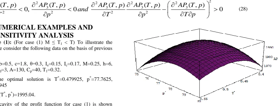
Example (1): (For case (1) M ≤ T1 < T) To illustrate the
model we consider the following data on the basis of previous study:
a=200, b=0.5, c=1.8, θ=0.3, Ie=0.15, Ic=0.17, M=0.25, h=6, δ=0.1, Cd=3, A=130, Cp=40, T1=0.32.
Then, the optimal solution is T*=0.479925, p*=77.7625, Q*=34.5945
and AP1(T *
, p*)=1995.04.
[image:5.595.86.565.508.691.2]The concavity of the profit function for case (1) is shown graphically in Figure 2.
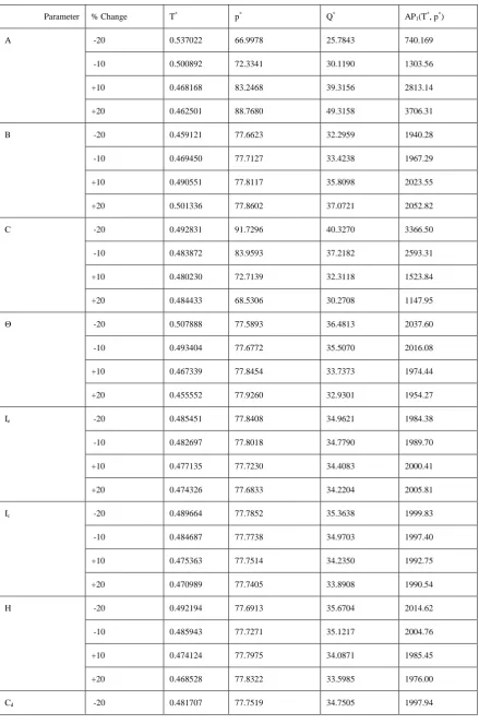
Table 1: The sensitivity analysis for case (1) is performed by changing the value of each of the parameters by
10%
and20%
, taking one parameter at a time and keeping the remaining parameters unchangedParameter % Change T* p* Q* AP
1(T*, p*)
A -20 0.537022 66.9978 25.7843 740.169
-10 0.500892 72.3341 30.1190 1303.56
+10 0.468168 83.2468 39.3156 2813.14
+20 0.462501 88.7680 49.3158 3706.31
B -20 0.459121 77.6623 32.2959 1940.28
-10 0.469450 77.7127 33.4238 1967.29
+10 0.490551 77.8117 35.8098 2023.55
+20 0.501336 77.8602 37.0721 2052.82
C -20 0.492831 91.7296 40.3270 3366.50
-10 0.483872 83.9593 37.2182 2593.31
+10 0.480230 72.7139 32.3118 1523.84
+20 0.484433 68.5306 30.2708 1147.95
Θ -20 0.507888 77.5893 36.4813 2037.60
-10 0.493404 77.6772 35.5070 2016.08
+10 0.467339 77.8454 33.7373 1974.44
+20 0.455552 77.9260 32.9301 1954.27
Ie -20 0.485451 77.8408 34.9621 1984.38
-10 0.482697 77.8018 34.7790 1989.70
+10 0.477135 77.7230 34.4083 2000.41
+20 0.474326 77.6833 34.2204 2005.81
Ic -20 0.489664 77.7852 35.3638 1999.83
-10 0.484687 77.7738 34.9703 1997.40
+10 0.475363 77.7514 34.2350 1992.75
+20 0.470989 77.7405 33.8908 1990.54
H -20 0.492194 77.6913 35.6704 2014.62
-10 0.485943 77.7271 35.1217 2004.76
+10 0.474124 77.7975 34.0871 1985.45
+20 0.468528 77.8322 33.5985 1976.00
-10 0.480813 77.7572 34.6722 1996.49
+10 0.479041 77.7678 34.5173 1993.59
+20 0.478162 77.7731 34.4401 1992.15
A -20 0.443718 77.5431 31.8732 2051.34
-10 0.462178 77.6550 33.2614 2022.64
+10 0.497035 77.8663 35.8780 1968.43
+20 0.513573 77.9666 37.1171 1942.70
Cp -20 0.511087 73.6465 41.7256 2615.13
-10 0.493806 75.7018 37.9337 2295.32
+10 0.469056 79.8307 31.6210 1713.90
+20 0.460971 81.9087 28.9470 1451.60
From sensitivity Table 1 the following inferences are drawn:
1. From Table 1 it is clear that the total profit per unit time AP1(T*,p*) increases or decreases with increase or decrease in the values of model parameters a, b and Ie, while AP1(T*,p*) decreases or increases with increase or decrease in the values of c, θ, Ic, h, Cd, A and Cp . The obtained results show that AP1(T*,p*) is highly sensitive to changes in a, c and Cp. It is moderately sensitive to changes in b, Ie, θ, Ic, h, Cd and A.
2. From Table 1 it is clear that
Q
* increases or decreases with increase or decrease in the values of model parameters a, b and A, whileQ
*decreases or increases with increase or decrease in the values of model parameters Ie, c, θ, Ic, h, Cd and Cp. The obtained results show thatQ
*is highly sensitive to changes in a and Cp. It is fairly sensitive to changes in b, c, θ, Ie, Ic, h and Cd.Example (2): (For case (2) T1< M ≤ T) We consider the
[image:7.595.77.518.70.313.2]following data in appropriate units: a=200, b=0.5, c=1.8, θ=0.3, Ie=0.15, Ic=0.17, M=0.4, h=6, δ=0.1, Cd=3, A=130, Cp=40, T1=0.32. Then, the optimal solution is T*=0.437287, p*=76.8656, Q*=31.9856 and AP2(T*, P)= 2137.46. The concavity of the profit function for case (2) is shown graphically in Figure 3.
[image:7.595.85.515.571.772.2]Figure 3. The concavity of the profit function (for case (2)) w.r.t. selling price and cycle length
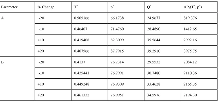
Table 2: The sensitivity analysis for case (2) is performed by changing the value of each of the parameters by
10%
and20%
, taking one parameter at a time and keeping the remaining parameters unchanged.Parameter % Change T* p* Q* AP
2(T*, p*)
A -20 0.505166 66.1738 24.9677 819.376
-10 0.46407 71.4760 28.4890 1412.65
+10 0.419408 82.3099 35.5644 2992.16
+20 0.407566 87.7915 39.2910 3975.75
B -20 0.4137 76.7314 29.5532 2084.12
-10 0.425441 76.7991 30.7480 2110.36
+10 0.449248 76.9309 33.4628 2165.35
C -20 0.439337 90.7672 36.1470 3550.83
-10 0.436382 83.0328 33.9014 2755.15
+10 0.441502 71.8413 30.2942 1649.25
+20 0.448791 67.6777 28.7547 1258.28
Θ -20 0.463019 76.7210 33.7641 2176.99
-10 0.449706 76.7946 32.8466 2157.00
+10 0.425666 76.9341 31.1754 2118.34
+20 0.414758 77.0003 30.4108 2099.63
Ie -20 0.457965 77.1366 33.4297 2100.62
-10 0.447758 77.0029 32.7189 2118.84
+10 0.426532 76.7242 31.2284 2156.50
+20 0.415468 76.5783 30.4452 2176.00
Ic -20 0.439318 76.8772 32.1423 2137.60
-10 0.438276 76.8712 32.0619 2137.53
+10 0.436349 76.8602 31.9133 2137.40
+20 0.435456 76.8551 31.8444 2137.33
H -20 0.448864 76.8075 32.9980 2155.71
-10 0.442965 76.8367 32.4842 2146.52
+10 0.431817 76.8941 31.5086 2128.53
+20 0.426542 76.9222 31.0494 2119.72
Cd -20 0.438968 76.8570 32.1324 2140.17
-10 0.438125 76.8613 32.0588 2138.81
+10 0.436454 76.8699 31.9129 2136.11
+20 0.435625 76.8742 31.8406 2134.77
A -20 0.397256 76.6158 28.9131 2199.77
-10 0.417757 76.7440 30.4874 2167.87
+10 0.455973 76.9814 33.4177 2108.35
+20 0.473915 77.0923 34.7914 2080.39
Cp -20 0.463193 72.8865 38.0963 2759.07
-10 0.448716 74.8732 36.7689 2430.82
+10 0.428556 78.8655 29.4405 1853.74
From sensitivity Table 2 the following inferences are drawn:
1. From Table 2 it can be shown that the total profit per unit time AP2(T*,p*) increases or decreases with increase or decrease in the values of model parameters a, b and Ie, while AP2(T
*
,p*) decreases or increases with increase or decrease in the values of c, θ, Ic, h, Cd, A and Cp . The obtained results show that AP2(T*,p*) is highly sensitive to changes in a, c and Cp. It is moderately sensitive to changes in b, Ie, θ, Ic, h, Cd and A.
2. From Table 2 it is clear that
Q
* increases or decreases with increase or decrease in the values of model parameter a, b and A, whileQ
*decreases or increases with increase or decrease in the values of model parameters Ie, c, θ, Ic, h, Cd and Cp. The obtained outcomes show thatQ
*is highly sensitive to changes in a and Cp. It is fairly sensitive to changes in b, c, θ, Ie, Ic, h and Cd.Example (3): (For case case (3) M > T) We consider the
following data in appropriate units: a=200, b=0.5, c=1.8, θ=0.3, Ie=0.15, Ic=0.17, M=0.6, h=6, δ=0.1, Cd=3, A=130, Cp=40, T1=0.32. Then the optimal solution is T*=0.533367, P*=76.6228, Q*=40.3092 and AP3(T
*
[image:9.595.315.560.159.277.2], p*)= 2335.76. The concavity of the profit function for case (3) is shown graphically in Figure 4.
Figure 4. The concavity of the profit function (for case (3)) w.r.t. selling price and cycle length
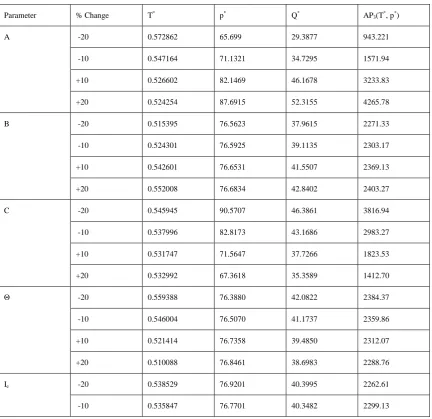
Table 3: The sensitivity analysis for case (3) is performed by changing the value of each of the parameters by
10%
and20%
, taking one parameter at a time and keeping the remaining parameters unchanged.Parameter % Change T* p* Q* AP3(T*, p*)
A -20 0.572862 65.699 29.3877 943.221
-10 0.547164 71.1321 34.7295 1571.94
+10 0.526602 82.1469 46.1678 3233.83
+20 0.524254 87.6915 52.3155 4265.78
B -20 0.515395 76.5623 37.9615 2271.33
-10 0.524301 76.5925 39.1135 2303.17
+10 0.542601 76.6531 41.5507 2369.13
+20 0.552008 76.6834 42.8402 2403.27
C -20 0.545945 90.5707 46.3861 3816.94
-10 0.537996 82.8173 43.1686 2983.27
+10 0.531747 71.5647 37.7266 1823.53
+20 0.532992 67.3618 35.3589 1412.70
Θ -20 0.559388 76.3880 42.0822 2384.37
-10 0.546004 76.5070 41.1737 2359.86
+10 0.521414 76.7358 39.4850 2312.07
+20 0.510088 76.8461 38.6983 2288.76
Ie -20 0.538529 76.9201 40.3995 2262.61
[image:9.595.83.516.344.763.2]+10 0.531069 76.4781 40.2811 2372.49
+20 0.528932 76.3358 40.2625 2409.32
H -20 0.545048 76.5255 41.4261 2358.32
-10 0.539109 76.5745 40.8576 2346.97
+10 0.527814 76.6706 39.7796 2324.70
+20 0.522438 76.7179 39.2678 2313.76
Cd -20 0.535070 76.6084 40.4717 2339.11
-10 0.534216 76.6156 40.3902 2337.44
+10 0.532523 76.6300 40.2286 2334.10
+20 0.531682 76.6372 40.1484 2332.43
A -20 0.507122 76.5016 38.2080 2385.74
-10 0.520409 76.5626 39.2719 2360.44
+10 0.546022 76.6822 41.3218 2311.68
+20 0.558394 76.7408 42.3115 2288.14
Cp -20 0.555727 72.6724 47.0640 2976.68
-10 0.54362 74.6468 43.5469 2647.11
+10 0.52486 78.6015 37.3118 2042.45
+20 0.51804 80.5841 34.5221 1767.00
From sensitivity Table 3 the following inferences are drawn:
1. From Table 3 it is clear that the total profit per unit time AP3(T*,p*) increases or decreases with increase or decrease in the values of model parameters a, b and Ie, even as AP3(T*,p*) decreases or increases with increase or decrease in the values of c, θ, h, Cd, A and Cp . The attained results show that AP3(T*,p*) is highly sensitive to changes in a, c and Cp. It is moderately sensitive to changes in b, Ie, θ, h, Cd and A.
2. From Table 3 it is clear that
Q
* increases or decreases with increase or decrease in the values of model parameters a, b and A, whereasQ
*decreases or increases with increase or decrease in the values of model parameters Ie, c, θ, h, Cd and Cp. The obtained results show thatQ
*is highly sensitive to changes in a and Cp. It is fairly sensitive to changes in b, c, θ, Ie, h and Cd.6.
CONCLUSION
In this study, an inventory model is developed with the facility of allowable delay in payment. The consumption rate is considered as a function of on hand inventory and selling price of the products. During the development of the model it is assumed that the on hand inventory affects the demand rate
only up to a certain time and after that only selling price affects the demand rate. According this theme three cases arise; all the cases are discussed and illustrated with the help of some numerical examples. Sensitivity analyses of system parameters clarify that a, c and Cp should be considered carefully.
There are several hopeful areas for further research. This model can be extended by considering probabilistic or inflation induced market demand rate. Another area for further research is that quantity discounted cash flow can be assumed.
7.
REFERENCES
[1] Levin, R.I., McLaughlin, C.P., Lamone, R.P., and Kottas, J.F., (1972). Production/Operations Management: Contemporary Policy for Managing Operating Systems. McGraw-Hill, New York.
[2] Silver, E.A., and Peterson, R., (1985). Decision Systems for Inventory Management and Production Planning. Second ed. John Wiley, New York.
[3] Goyal, S.K., (1985). Economic order quantity under conditions of permissible delay in payments. Journal of the Operational Research Society, 36(4), 335–338. [4] Gupta, R., and Vrat, P., (1986). Inventory model for
[5] Mandal, B.N., and Phaujdar, S., (1989). An inventory model for deteriorating with stock dependent consumption rate. Opsearch, 26, 43–46.
[6] Datta, T.K., and Pal, A.K., (1990). Deterministic inventory systems for deteriorating items with inventory-level-dependent demand rate and shortages. Opsearch, 27, 167–176.
[7] Padmanabhan, G., and Vrat, P., (1995). EOQ models for perishable items under stock dependent selling rate. European Journal of Operational Research, 86, 281–292. [8] Aggarwal, S.P., and Jaggi, C.K., (1995). Ordering
policies of deteriorating items under permissible delay in payments. Journal of the Operational Research Society, 46(5), 658–662.
[9] Jamal, A.M.M., Sarker, B.R., and Wang, S., (1997). An ordering policy for deteriorating items with allowable shortages and permissible delay in payment. Journal of the Operational Research Society, 48, 826–833.
[10]Urban, T.L., and Baker, R.C., (1997). Optimal ordering and pricing policies in a single-period environment with multivariate demand and markdowns. European Journal of Operational Research, 103, 573–583.
[11]Datta, T.K., and Paul, K., (2001). An inventory system with stock-dependent, price-sensitive demand rate. Production Planning & Control, 12, 13–20.
[12]Chang, H.J., and Dye, C.Y., (2001). An inventory model for deteriorating items with partial backlogging and permissible delay in payments. International Journal of Systems Science, 32, 345–352.
[13]Teng, J.T., (2002). On the economic order quantity under conditions of permissible delay in payments. Journal of the Operational Research Society, 53, 915–918. [14]You, P.S., (2005). Inventory policy for products with
price and time dependent demand. Journal of the Operational Research Society, 56, 870–873.
[15]You, P.S., and Hsieh, Y.C., (2007). An EOQ model with stock and price sensitive demand. Mathematical and Computer Modelling, 45, 933–942.
[16]Sana, S.S., and Chaudhuri, K.S., (2008). A deterministic EOQ model with delays in payments and price-discount offers. European Journal of Operational Research, 184, 509–533.
[17]Chang, C.T., Chen, Y.J., Tsai, T.R. and Wu S.J., (2010). Inventory models with stock- and price dependent demand for deteriorating items based on limited shelf space. Yugoslav Journal of Operations Research, 20, 55– 69.
[18]Khanra, S., Ghosh, S.K. and Chaudhuri, K.S., (2011). An EOQ model for a deteriorating item with time dependent quadratic demand under permissible delay in payment. Applied Mathematics and Computation, 218, 1, 1-9. [19]Teng, J. T., Min, J., and Pan, Q., (2012). Economic order
quantity model with trade credit financing for non-decreasing demand. Omega, 40(3), 328-335.