Munich Personal RePEc Archive
Predictive Performance of Conditional
Extreme Value Theory and Conventional
Methods in Value at Risk Estimation
Ghorbel, Ahmed and Trabelsi, Abdelwahed
Institut Supérieur de Gestion, Laboratoire BESTMOD, Université
de Tunis
31 March 2007
Online at
https://mpra.ub.uni-muenchen.de/3963/
Predictive Performance of Conditional Extreme Value
Theory and Conventional Methods in Value at Risk
Estimation
Ahmed Ghorbel, Abdelwahed Trabelsi 1
Institut Supérieur de Gestion, Laboratoire BESTMOD, Université de Tunis 41, avenue de la liberté, le Bardo 2000, Tunis, Tunisie
March 31, 2007
Abstract
This paper conducts a comparative evaluation of the predictive performance of various Value at Risk (VaR) models such as GARCH-normal, GARCH-t, EGARCH, TGARCH models, variance-covariance method, historical simulation and filtred Historical Simulation, EVT and conditional EVT methods. Special emphasis is paid on two methodologies related to the Extreme Value Theory (EVT): The Peaks over Threshold (POT) and the Block Maxima (BM). Both estimation techniques are based on limits results for the excess distribution over high thresholds and block maxima, respectively. We apply both unconditional and conditional EVT models to management of extreme market risks in stock markets. They are applied on daily returns of the Tunisian stock exchange (BVMT) and CAC 40 indexes with the intension to compare the performance of various estimation methods on markets with different capitalization and trading practices. The sample extends over the period July 29, 1994 to December 30, 2005. We use a rolling windows of approximately four years (n= 1000 days). The sub-period from July, 1998 for BVMT (from August 4, 1998 for CAC 40) has been reserved for backtesting purposes. The results we report demonstrate that conditional POT-EVT method produces the most accurate forecasts of extreme losses both for standard and more extreme VaR quantiles. The
conditional block maxima EVT method is less accurate.
Keywords : Financial Risk management, Value-at-Risk, Extreme Value Theory,
Conditional EVT, Backtesting
1 . Introduction
Over the last seventeen years, risk management gained great importance due to increase in the volatility of financial markets and a desire of less volatile financial markets and less fragile financial system. Value-at-Risk models have been implemented throughout the financial industry and by non-financial corporations as well. VaR has became the key and standard measure that financial analysts use to quantify risk. It is defined as the maximum potential loss in value of an asset or a portfolio with a given probability over a certain horizon. It measures the potential loss on a portfolio that would result if relatively large adverse price movement were to occur. It is a number that indicates how much a financial institution or an investor can lose with a given probability over a given time horizon. The VaR s great popularity originates from the aggregation of several components of risk at firm and market into a single number. The Basel Commitee on banking supervision (1996) at the bank for international settlements imposes to financial institutions such as banks and investment firms to meet capital requirement based on VaR estimates. It is crucially interesting to provide accurate estimates. If risk is not properly estimated, these can lead to a sub-optimal allocation.
VaR works on multiple levels, from the position-specific micro level to the portfolio-based macro level. It has become a common language for communication about aggregate risk taking, both within and outside an organisation.
A key element to VaR calculation is the distribution function we choose for the price change of an asset or portfolio. To calculate VaR, we can choose from three main methods: parametric, historical simulation and Monte Carlo simulation. Each method has some strengths and some weaknesses, and together offer a more comprehensive perspective of risk. The parametric method estimates VaR with equation that specifies parameters such as volatility and correlation, it is accurate for traditional assets and linear derivatives but less accurate for non linear derivatives and for skewed distributions. The Historical Simulation estimates VaR by reliving history; takes actual historical rates and revalues positions for each change in the market. Monte Carlo simulation method estimates VaR by simulating random scenarios and revaluing positions in the portfolio. The last two methods are appropriate for all types of instruments, linear and non linear and are mechanically identical in that they both revalue instruments, given changes in market rates. The difference lies in how they generate market scenarios. HS method takes actual past market movements as scenarios while MC method generates random hypothetical scenarios.
December 30, 2005. We use a rolling windows of approximately four years (n= 1000 days). The sub-period from July, 1998 for BVMT index (and from August 4, 1998 for CAC 40) has been reserved for backtesting purposes.
The present paper is organized as follows. The EVT, conditional EVT and conventional VaR estimation methods are introduced in section 2. Section 3 describes the evaluation framework for VaR estimation. Empirical results and predictive performance evaluation of several models are presented in section 4. We conclude afterwards.
2 . VaR models
VaR has become a standard for measuring and assessing risk. It is defined as a quantile of the distribution of returns (or losses) of asset or portfolio in question. It is defined also as the predicted worst-case loss at a specific confidence level over a certain period of time. Some practitioners prefer to make in consideration the negative of this quantile, so that higher values of VaR correspond to higher level of risk.
Formally, Let rt log(pt/pt 1) be the returns at time t where ptis the price of an asset (or
portfolio) at time t. We denote the (1-p)% quantile estimate at time t for a one-period-ahead return as VaR (p), so that
p p VaR
rt t( ))
Pr(
The VaR s popularity originates from the aggregation of several components of risk at firm and market into a single number.
More formally, VaR is calculated based on the following equation
t
t F p
VaR 1( )
given that F-1(p) is the corresponding quantile of the assumed distribution and t is the
forecast of the conditional standard deviation at time t-1.
2.1 Variance- covariance method
The variance-covariance method is one of the simplest approach among various models used
to estimate the VaR. let as assume that returns can be written as: rt t t where thas a
distribution function F with zero mean and variance t2. The VaR can be calculated as
q t t
t F q
VaR 1( ) (1)
where F 1(q) is the qth quantile value of an unknown distribution function F. We can
estimate t and t2by the sample mean and the sample variance by
n
i t
t r
n 1 1
2
1 2
) ( 1
1 n
i
t t
t n r
2.2 Historical simulation
An approach to VaR modelling is to estimate the quantile nonparametrically. A Conventional way is to use the historical simulation. This method is powerful because of its simplicity and its relative lack of theoretical baggage. It assume that the distribution of return will remain the same in the past and in the future and hence historical returns will be used in the forecast of Value-at-risk.
VaRp Quantile yt nt 1,100p (2)
This method need not to make distributional assumptions (although parameter fitting may be performed on the resulting distribution). It accommodates non-normal distributions and therefore it accounts for fat tails and non-zero skewness. HS provides a full distribution of potential portfolio values, not just a specific percentile. The key assumption of this method is that the series under consideration is IID. For more turmoil periods, it can turn out to be a very bad measure of risk since risk can change significantly. VaR estimate using this simple approach is extremely sensitive to the choice of the sample length n. If n is too large, the most recent returns, that probably can describe better the future, have the same weight with the earliest observations. If n is too small, then a few or an insufficient extreme events will be observed and possibility to incorporate tail risk became more difficult.
2 .3 Filtred Historical simulation
This method consists to combine volatility models (parametric) and historical simulation method (non-parametric). Such combination might lessen the problematic use of the traditional approaches, since it can accommodate the volatility clustering, the observed fat tails and the skewness of the empirical distribution.
By using the quantiles of the standardized residuals and the conditional standard deviation forecast from a volatility model, the VaR number is calculated as:
VaRp t Quantile t nt 1,100p t 1 (3)
In our empirical investigation, we assume that the volatility estimates and the corresponding quantiles are being generated via a GARCH(p,q) process.
2.4 GARCH models2
We assume that the return series is decomposed into two parts, the predictive and
unpredictable component, rt t t where t is the conditional mean and tis the
unpredictable part or innovation process. The conditional mean return can be expressed as a s-th order autoregressive process, AR(s):
s
i i t
t r
1
0 (4)
The unpredictable component t can be expressed as an ARCH process as follow:
t t
t z
2
whereztis a sequence of independently and identically distributed random variables with zero
mean and unit variance. The conditional variance on information at time t-1 of innovations t
is 2
t .
2.4.1 GARCH model:
Engle (1982) introduced the ARCH (p) model and expressed the conditional variance as a linear function of the past p squared innovations
p
i
i t i t
1 2 0
2
The conditional variance will be positive, if 0 0 and i 0 for i=1,2, ,p. Bollerslev
(1986) proposed a generalization of the ARCH model, the GARCH(p,q) model. Generalized AutoRegressive Conditional Heteroskedasticity model permits to express the conditional variance as a linear function of lagged squared error terms and lagged conditional variance terms.
2
1 1
2 0
2
j t q
ji j p
i
i t i
t (5)
where 0 0 and i 0 for i=1,2, ,p. If 1
1 1
p
i j q
i
i , the process tis covariance
stationary and its unconditional variance is equal to
1
1 1
0 2
q
i j p
i i t
The GARCH (p,q) model is successfully captures several characteristics of financial time series, such as thick tailed returns and volatility clustering.
2.4.2 EGARCH model:
In the GARCH model, the signs of residuals or shocks have no effects on conditional volatility only squared residuals enter in the conditional variance equation. However, a stylized fact of financial volatility is that bad news (negative shocks) tends to have a larger impact on volatility than good news (positive shocks). Bad news tends to drive down the stock price, thus increasing the leverage of the stock and the stock will be more volatile (Black , 1976) .
Nelson (1991) proposed the following exponential GARCH (EGARCH) model to allow for leverage effects:
q
j
j t j p
i t i
i t i i t i
t In
In
1
2
1 0 2
) ( )
( ( 6)
In contrast to the GARCH model, no restrictions need to imposed on the model estimation, since the logarithmic transformation ensures that the forecasts of the variance are non-negative.
Note that when t i is positive or there is a good news, the total effect of t i is (1 i) t i ; in
2.4.3 TGARCH model:
Another GARCH model that is capable of modelling leverage effects is the threshold GARCH (TGARCH) model or also known as the GJR model (Glosten, Jagannathan, and Runkle, 1993) which has the following form:
2 1 1 2 1 2 0 2 j t q ji j p i i t i t i p i i t i
t S (7)
where 0 0 0 1 i t i t i t if if S
That is, depending on whether innovation t iis above or below the threshold value of 0, t2i
has different effects on the conditional variance: if innovation is negative, the total effects are
2 )
( i i t i ; when innovation is positive the total effect are given by i t2i.
Engle (1982) assumed that standardized residual zt is normally distributed.
) 2 exp( ) 2 ( ) ( 2 ) 2 / 1 ( t t D
However, given the well known fat tails in financial time series, it may be more desirable to use a distribution which has fatter tails than the normal distribution. Bollerslev (1987) proposed
to use the standardized symetric t-distribution with 2 degrees of freedom with a density
given by 2 1 2 ) 2 1 ( ) 2 ( ) 2 / ( ) 2 / ) 1 (( ) , ( v t t v v v v v D
where (.) is the gamma function.
The one-step ahead conditional variance forecast t2, for the GARCH (p,q) model is given
by 2 1 1 2 0 2 j t q ji j p i i t i
t (8)
For the EGARCH(p,q) model, one step-ahead conditional variance forecast is given by
q j j t j p
i t i
i t i i t i t In In 1 2 1 0 2 ) ( )
( (9)
In the case of TGARCH (p,q) model, we forecast conditional variance using the following expression 2 1 1 2 1 2 0 2 j t q ji j p i i t i t i p i i t i
t S (10)
In our empirical study, we will evaluate the predictive performance of GARCH-N model in which the error term is assumed normally distributed, GARCH-t model in which we assume that the error term follows a student-t distribution with v degrees of freedom, TGARCH and
EGARCH models not in an econometric laboratory but in a risk management environment3.
3
2.5 Extreme Value Theory
Extreme Value Theory is a classical topic in probability theory. EVT is a powerful and yet fairly robust framework in which to study the tail behaviour of a distribution. It can be conveniently thought as a complement to the cetral limit theory: while the latter deals with fluctuations of cumultative sums, the formers deals with fluctuations of sample maxima. The main result is due to Fisher and Tippet (1928), who specify the form of the limit distribution appropriately normalised maxima.
There have been a number of extreme value studies in the finance literature in recent years. De Haan, Jansen, Koedijk and de Vries (1994) study the quantile estimation using extreme value theory. Mc Neil (1998) study the estimation of the tails of loss severity distributions and the estimation of the quantile risk measures for financial data using extreme value theory. Embrechts et al. (1998) overview the extreme value theory as a risk management tool. Muller et al. (1998) and Pictet et al. (1998) study the probability of exceedences and compare them with GARCH models for the foreign exchange rates. Mc Neil (1999) provides an extensive overview of the extreme value theory for risk managers. One year after, Mc Neil and Frey develop a new approach in two steps that permits to estimate the tail- related risk measures for heteroskedastic financial time series, a such method is a combination between GARCH models and EVT method. Some applications of EVT to finance and insurance can be found in Embrechts, Klueppeelberg and Mikosch (1997) and Reiss and Thomas (1997).
In the following , we present two approaches to study extreme events. The first one is a direct modelling of the distribution of minimum or maximum realizations. The other one is modelling the exceedances of a particular threshold. In addition, we present Mc Neil et al (2000) approach called conditional EVT and used to estimate tail-related risk measures in the case of heteroskedastic financial time series.
2.5.1 The block maxima method
Let X1, X2, X3, , X be a sequence of independently and identically distributed random n
variables with a common distribution function CDF F(x) Pr(Xt x) which has mean
(location parameter) µ and variance (scale parameter) 2. Throughout this work, a loss is
treated as a positive number and extreme events occur when losses take values in the right tail of the loss distribution F. Under the block maxima method, the data are divided into k blocks with n observations in each block corresponding to n trading intervals. Let the sample maxima
of X denote the worst-case loss in a sample of n losses. From the iid assumption, the CDF n
of Mn is given by
X n
n
i
i n
n x X X X x X x F x
M ) Pr(max( , ,..., ) ) Pr( ) ( ) Pr(
1 2
1 (11)
n
F is assumed to be unknown and the empirical distribution function is often a very poor
estimator of Fn(x). Fisher and Tippet (1928) have shown that for X that are independent and t
drawn from the same non-degenerate distribution function H such that
limPr y lim F c y d H(y)
c d M
n n n
n n
n n
Then H belongs to one of the three standard extreme value distributions, regardless of the original distribution of the observed data.
Fréchet:
0 ,
0 ),
exp(
0 ,
0 )
(
x x
x x
Weibull:
0 ,
1
0 ,
0 )],
( exp[
) (
x x x
x
Gumbel : ( x) exp( exp( x)), x
Fréchet and Weibull distributions attain the shape of a Gumbel distribution when the tail index
parameter goes to and , respectively. By taking the reparameterization 1 , due
to Jenkin (1955) and Von Mises (1936), these three extreme value distributions can be represented in an unified model with a single parameter
0 ,
) exp( exp
0 1
, 0 ,
) 1 ( exp
) (
/ 1
if x
x if
x
x
H (13)
The parameter 1
is a shape parameter and determines the tail behaviour of H . The
parameter is called the tail index if >0. This representation is known as the generalized
extreme value distribution (GEV). The tail behaviour of the distribution F of the underlying
data determines the shape parameter of the GEV distribution. If the tail of F declines
exponentially, then H is of the Gumbel type and =0. Normal, log-normal, exponential and
gamma distributions are thin tailed distributions and are in the domain of attraction of the Gumbel type. For these distributions, all moments usually exist. Distributions in the domain of attraction of the Fréchet type ( >0) include fat tailed distributions like the Stundent-t, Cauchy, Pareto, and mixture distributions. For these distributions, not all moments are finite. If the tail
of F is finite then H is of the weibull type and <0. Distributions in the domain of attraction
of the weibull type include distributions with bounded support such as uniform and beta distributions. All moments exist for these distributions.
The Fisher-Tippet Theorem is the analog of the Central Limit Theorem for extreme values. Whereas the Central Limit Theorem applies to normalized sums of random variables, the Fisher- Tipett Theorem applies to standardized maxima of random variables.
) ( )
(z H x µ H , , x
H µ
For n large, the Fisher- Tippet theorem may then interpreted as follows
) ( Pr
)
Pr(Z z M µ z H z
n n n n
Letting x nz µnthen
Pr(M x) H , , x µ H , , (x)
n n µ n n µ
n (14)
This result is used in practice to make inferences about the maximum loss Mn.
The parameters of the GEV distribution ( , µn and n) are estimated by fitting the GEV
distribution to the data. The likelihood function for the parameters of the GEV distribution is
constructed from the sample of block maxima M1, M2, ...Mk . We assume that each block
is of size n sufficiently large so that the Fisher-Tppet Theorem holds.
i
i µ
H Max In h x
MaxL ( , , ) ( , , ( ))
where / 1 1 / 1 ,
, 1 exp 1
1 )
( i i
i µ x µ x x h
is the density function of the GEV distribution if 0 and 1 xi 0
. and / 1 1 1 1 1 ) / 1 1 ( ) ( ) , , ( k i i k i i H x µ x In kIn
L (15)
is the log function assuming iid observations from a GEV distribution whith 0.
For the case where 0, the likelihood is given by
k i i k i i H x µ x kIn L 1 1 exp ) ( ) ,
By inverting equation ( ), we can go from asymptotic GEV distribution of maxima to the distribution of the observations themselves and we can get an expression for (unconditional)
p
VAR quantiles associated with a given probability p
, 1 1 1 1 1 1
k In µ
k H
R
VaRp nk (17)
where , and have been substituted by their maximum likelihood estimates. If
observations Xi are independent then
) ( ) ,...,
Pr( 1
1 X1 Rn,k Xn Rn,k Fn Rn,k k
In the case of iid series, The (1-1/k) quantile,Rn,k, for the distribution of maxima
n
M corresponds to the 1 (1/k)1/n quantile of the marginal distribution of Xi. Suppose for
example that we consider our model for annual (260 days) maxima. Then, the return that we expect to be exceeded once every 30 years, the 30 year return level corresponds to the
99987 , 0 30
/ 1
1 (1/260) quantile.
We have only considered the case of stationary and independently distributed random variables. In the case of non-iid variables which are supposed to hold in most financial markets, we can fit a slightly modified GEV distribution to stationary series that show that show the kind of clustering behaviour.
For iid series, we can easily calculate the distribution of the sample maxima from a distribution F of sample observations
n X
M F
F [ ]
As this case is unrealistic for financial time series, we extend the asymptotic proprieties of
maxima derived for an iid variable to the non-i.i.d case. Let (Xn) be a stationary variable with
marginal distribution F and (X~n ) an associated independent process which have the same
marginal distribution F and letM~n max(X~1,....,X~n). We define a new parameter 0,1
called extremal index such that
n X k n n k n n k
n n
M P M R P M R F R F
F ( , ) (~ , ) ( , )
This means that the maximum of n observations from the non-i.i.d series have behaviour like
the maximum of n observations from the associated iid variables. can be interpreted as the
reciprocal of the mean cluster size and n as counting the number of pseudo-independent
clusters in n observations. The asymptotic distribution of maxima for non-iid series is in fact a
GEV distribution that converge in probability to H (x). The GEV distributions for iid and
non-iid series have the same tail index, because raising H(x) to the power only affects scale
as a reciprocal of the mean cluster size and n as counting the number of pseudo-independent clusters in n observations. The extremal index can be estimated asymptotically as
) / 1 (
) / 1 ( 1
nk N In
k K In n
u u
(18)
where Nu is the number of observations that exceed a certain high threshold, Ku is the number
of blocks in which this threshold is exceeded, and k and n, which should be large, are the number of blocks and length of these blocks respectively.
2.5.2 The POT method
The distribution function Fuis called the conditional excess distribution function (cedf) an is
defined as the conditional probability:
Fu(y) P(X u y/X u), 0 y xF u (19)
where X is a random variable, u is a given threshold, y=x-u is the excess over u and xF is the
right endpoint of F.
0 1
0 )
1 ( 1 ) (
1
,
if e
if y
y G
y
(20)
for 0 y xF u. is the tail index.
F(x) (1 F(u))Fu(y) F(u) (21)
The function F(u) can be estimated non parametrically by
n N n u
where n is the total
number of observations and N represents the number of exceedences over the threshold uu 4.
After replacing Fu(y) by G , (y), we get the following estimate for F(x):
( ) (1 (1 ( )) ) (1 ) 1 (1 (x u))
n N n
N u
x n
N x
F u u
u
(22)
By inverting this expression, we get an expression for (unconditional) VARp quantiles
associated with a given probability p:
(( p) 1)
N n u
VAR
u
p (23)
2.5.3 The Conditional EVT approach
To obtain value-at-risk estimates, we follow MC Neil and Frey s (2000) two-step estimation
procedure called conditional EVT5:
Step 1: Fit a GARCH-type model to the return data by quasi-maximum likelihood. That is, maximize the log-likelihood function assuming normal innovations.
Step 2: Consider the standardized residuals computing in step 1 to be realizations of a strict white noise process and use extreme value theory (EVT) to model the tail of innovations using
EVT and estimate the quantiles of innovations for q 0.95.
We assume that the dynamic of log-negative returns can be modelled by
rt t tZt (24)
where s i i t t r 1
0 , i are parameters, rt iare lagged returns and Ztare iid innovations
with zero mean and unit variance and marginal distribution FZ(z). We assume that the
conditional variance t2of the mean-adjusted series t rt t follows a GARCH (p,q)
process: 2 1 1 2 0 2 j t q ji j p i i t i
t (25)
The conditional mean is given by
s i i t t r 1
0 , and the likelihood function of a sample
of m iid observations for a GARCH model with normal innovations is given by
m t t t t m t t r m L 2 2 2 ) ( 2 1 ) log( 2 1 ) 2 log( 2 )
( (26)
After maximizing, we can obtain parameter estimates and compute standardized residuals to check the adequacy of the GARCH modelling and to use in stage 2 of the method. They are calculated as 1 2 2 2 1 1 1 2
1, ,...., ) , ,...
( t t
m t m t m t m t m t m t t m t m t r r r z z
z (27)
The one-step forecast for the conditional variance in t+1 is given by
2 1 1 1 2 1 0 2
1 t j
q ji j p i i t i
t (28)
where t
r
t t . The one-step-ahead VaR forecasts is given byVaRp t 1VaR(Z)p (29)
5
where VaR(Z)pis given by equation 23 (or by equation 17) applied to negative standardized residuals to obtain VaR forecasts with conditional EVT-POT method ( conditional block
maxima method)6.
3 . Statistical evaluation tests:
Our objective is to evaluate the adequacy of the realized VaR forecasts in a risk management environment. It is well know that there are many sources of error in VaR figures: Sampling errors, data problems, inappropriate specification, model error, ect. All these factors will cause our estimate often to be biased. Various methods and tests have been suggested for evaluating VaR model accuracy. In this paper, statistical adequacy will be tested based on Kupiec s and Christoffersen s backtesting measures.
3 .1 Unconditional coverage:
Let It 1 be a sequence of VaR violations that can be described as:
t t t
t t t
t
VaR y
if
VaR y
if I
/ 1 1
/ 1 1
1
0 1
and therefore
T
t t
I N
1
be the number of days over a T period that the portfolio loss was
greater than the VaR forecast.
The failure number follows a binomial distribution and consequently the appropriate likelihood ratio statistic, under the null hypothesis that the exception frequency equals to the excpected one (N/T=p) is:
uc 2 [(1 )T N( )N] 2In[(1 p)T N pN]~ 2(1)
T N T
N In
LR (30)
This test can reject a model that has generated too many or too few VaR violations. As stated by Kupiec, this can reject a model for both high and low failures but its power is generally poor especially for high confidence levels, it can not indicate an inadequate model, even if the difference between the observed and the expected failure is significant.
.
3 .2 Conditional coverage:
A more complete test was made by Christoffersen (1998), which jointly examines the conjecture that the total number of failures is statistically equal to the expected one and the VaR violations are independent. The main advantage of this test that it takes account of any conditionality in forecasts: if volatilities are low in some period and high in others, the forecast should respond to this clustering from distribution event. Under the null huypothesis that an expectation occurring is independent on what happened the day before and the expected proportion of violations is equal to p, the appropriate likelihood ratio is given by
2 [(1 )T N( )N] 2 [(1 01) 00 01n1(1 11) 10 11n11]~ 2(2)
cc
n à
n In
p p In
LR (31)
where nijis the number of observations with value i followed by j, for i, j =0,1 and
j ij ij ij
n n
Table 1
Descriptive statistics on stock returns
Index Sample Mean stdev Min Max JB Q(12) Q(24) Q²(12) Q²(24) LM
In sample
0.019 0.431 3.93 2 12083.8 495.3 593.6 295.2 327.3 78.5
BVMT
All sample
0.039 0.692 3.93 3.62 1572.5 570.23 603.0 2140.0 2434.4 776.3
In sample
0.067 1.131 4.37 6.1 67.7 18 34.59 69.9 84.5 50.5
CAC40
All sample
0.028 1.393 7.678 7 813.0 26.3 47.4 1739.1 2876.9 521.9
Mean, standard deviation, min and max are in percent. JB is the Jarque-Bera test for normality. Q(.) are the Ljung-Box tests for returns and for squared returns. LM refers to the Engle (1982) Lagrange Multiplier test for the presence of ARCH effect at lag 12.
j ij ij ij
n n
are the corresponding probabilities. i,j=1denotes that an expectation has been made, while i,j=0 indicates the opposite. If the sequence of values is independent, then the probabilities to observe or not a VaR violation in the next period must be equal, which can be written more
formally as 01 11 p. This test can reject a VaR model that generates either too many or
too few clustered violations, but it needs several observations to became more accurate.
4. Empirical Results
1 .4 Data and descriptive statistics
The data set is the daily closings of Tunis stock Exchange (BVMT) index and CAC 40 for the same period from July 29, 1994 to December 30, 2005. There are observations 2868 in data set for BVMT index and 2890 for CAC 40 index. The period July 24, 1998 to December 30, 2005 has been reserved for backtesting the predictive performance of alternative models for BVMT index. For CAC 40 index, the period reserved for backtesting cover Aout 4, 1998 to
December 30, 2005. The daily returns are defined by rt log(pt/pt 1) where ptis the price of
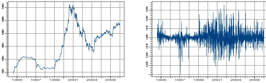
an asset (or portfolio) at time t. In fig.1, the level of BVMT index and the corresponding daily returns are presented. The sample histogram of negative BVMT returns (returns multiplied with -1) is presented in Fig.2.
All computations shown hereafter were carried out with finmetrics module of S-Plus 6.1.
1995 1997 1999 2001 2003 2005
4
0
0
6
0
0
8
0
0
1
0
0
0
1
2
0
0
1
4
0
0
1995 1997 1999 2001 2003 2005
-0
.0
3
-0
.0
2
-0
.0
1
0
.0
0
0
.0
1
0
.0
2
0
.0
3
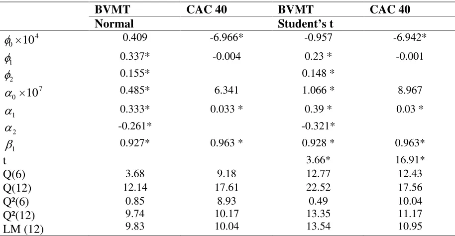
[image:15.595.95.526.589.724.2]Table 2
Parameters estimates of AR-GARCH models for THE two index, as well as statistics on the standardized residuals.
BVMT CAC 40 BVMT CAC 40
Normal Student s t
0 4
10 0.409 -6.966* -0.957 -6.942* 1 0.337* -0.004 0.23 * -0.001 2 0.155* 0.148 *
0 7
10 0.485* 6.341 1.066 * 8.967 1 0.333* 0.033 * 0.39 * 0.03 * 2 -0.261* -0.321*
1 0.927* 0.963 * 0.928 * 0.963*
t 3.66* 16.91*
Q(6) 3.68 9.18 12.77 12.43
Q(12) 12.14 17.61 22.52 17.56
Q²(6) Q²(12) LM (12)
0.85 9.74 9.83
8.93 10.17 10.04
0.49 13.35 13.54
10.04 11.17 10.95
* Significance at 95% level. Q(.) are the Ljung-Box tests. LM is the Lagrange multiplier test.
-0.040 -0.032 -0.024 -0.016 -0.008 0.000 0.008 0.016 0.024 0.032 0.04 r
0 20 40 60 80 100
Fig. 2: Histogram of daily negative BVMT returns (losses)
1995 1997 1999 2001 2003 2005
2
0
0
0
2
5
0
0
3
0
0
0
3
5
0
0
4
0
0
0
4
5
0
0
5
0
0
0
5
5
0
0
6
0
0
0
6
5
0
0
1995 1997 1999 2001 2003 2005
-0
.0
6
-0
.0
4
-0
.0
2
0
.0
0
0
.0
2
0
.0
4
0
.0
6
[image:16.595.140.473.387.516.2] [image:16.595.102.507.569.714.2]
The descriptive statistics for daily returns of each index are presented in table 1. These statistics include the mean, standard deviation, median, maximum, minimum, Jarque-Bera statistics and Ljung-Box tests for raw and squared returns. The Jarque-Bera statistic indicate that daily returns for the two markets are not normally distributed. On the basis of Ljung-Box Q statistic and for raw returns series, the hypothesis that all correlation coefficients up to twelve and up to twenty four are jointly zero is rejected for the two markets. Therefore, we can conclude that two return series present some linear dependence in returns. In addition, the statistically significant serial correlations in squared returns imply that there is non linear dependence in return series. This indicates volatility clustering and a GARCH type modelling should be considered in VaR estimations.
4.2 In-sample evidence
The first step was to fit the model in Eqs. 24 and 25 to each return series. To identify the most adequate AR-GARCH model for each time series, we employ the Akaike criterion (AIC). For BVMT return series, we choose the AR(2)- GARCH(2,1) model. For CAC 40 returns, as in previous studies, we choose the AR(1)-GARCH(1,1) model. Parameter estimates for the models selected were obtained by the method of quasi-maximum likelihood and the log-likelihood function of the data was constructed by assuming that innovations are conditionally distributed as Gaussian. For the AR-GARCH models with normal distributed and with t-distributed errors, maximum likelihood estimates as well as some statistics on the standardized residuals are presented in table 2.
0 200 400 600 800 1000
-0
.0
3
-0
.0
1
0
.0
1
0
.0
3
0 200 400 600 800 1000
0
.0
0
5
0
.0
1
0
0
.0
1
5
0
.0
2
0
0
.0
2
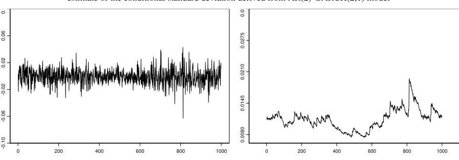
[image:17.595.82.530.387.530.2]5
Fig. 4: 1000 day excerpt from series of negative log returns on BVMT index; plot in the right shows
estimate of the conditional standard deviation derived from AR(2)-GARCH(2,1) model
0 200 400 600 800 1000
-0
.1
0
-0
.0
6
-0
.0
2
0
.0
2
0
.0
6
0
.1
0 200 400 600 800 1000
0
.0
0
8
0
0
.0
1
4
5
0
.0
2
1
0
0
.0
2
7
5
0
.0
3
Fig. 5: 1000 day excerpt from series of negative log returns on CAC 40 index; plot in the right shows
[image:17.595.79.527.564.720.2]Lag
A
C
F
0 10 20 30
0 .0 0 .2 0 .4 0 .6 0 .8 1 .0
Series : r
Lag
A
C
F
0 10 20 30
0 .0 0 .2 0 .4 0 .6 0 .8 1 .0
Series : r^2
Lag
A
C
F
0 5 10 15 20 25 30
0 .0 0 .2 0 .4 0 .6 0 .8 1 .0
Series : residuals
Lag
A
C
F
0 5 10 15 20 25 30
0 .0 0 .2 0 .4 0 .6 0 .8 1 .0
[image:18.595.83.509.76.335.2]Series : residuals^2
Fig. 6: Correlograms for the raw data (BVMT) and their squared values as well as for the residuals and squared residuals.
Lag
A
C
F
0 10 20 30
0 .0 0 .2 0 .4 0 .6 0 .8 1 .0
Series : r
Lag
A
C
F
0 10 20 30
0 .0 0 .2 0 .4 0 .6 0 .8 1 .0
Series : r^2
Lag
A
C
F
0 5 10 15 20 25 30
0 .0 0 .2 0 .4 0 .6 0 .8 1 .0
Series : resid
Lag
A
C
F
0 5 10 15 20 25 30
0 .0 0 .2 0 .4 0 .6 0 .8 1 .0
Series : resid^2
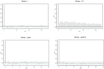
Fig. 7: Correlograms for the raw data (CAC 40) and their squared values as well as for the residuals and squared residuals.
[image:18.595.83.514.378.666.2]In Fig.6 and 7, we plot correlograms for the raw data and their squared values as well as for the residuals and squared residuals. While the raw data are clearly not iid, this assumption may be tenable for residuals.
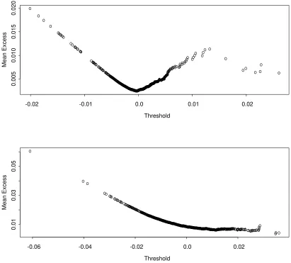
The mean excess plots for the BVMT and CAC 40 data are illustrated in Fig. 87.
A simple graphical technique infers the tail behaviour of observed losses is to create a qq-plot using the exponential distribution as a reference distribution. If the excesses over thresholds are
from a thin- tailed distribution, then the GPD is exponential with 0 and the qq-plot should
be linear. If the qq-plot is non-linear this indicate either bounded tails ( 0) or fat-tailed
behaviour ( 0). Fig.9 shows qq- plots with exponential references distribution for the
BVMT negatives returns and the CAC 40 negatives returns over the threshold u. There is a slight departure from linearity for the negative CAC 40 returns and a large departure from linearity for the negative CAC 40 index.
A simple graphical technique infers the tail behaviour of observed losses is to create a qq-plot using the exponential distribution as a reference distribution. If the excesses over
thresholds are from a thin- tailed distribution, then the GPD is exponential with 0 and the
qq-plot should be linear. If the qq-plot is non-linear this indicate either bounded tails ( 0) or
fat-tailed behaviour ( 0). Fig.9 shows qq- plots with exponential references distribution for
the BVMT negatives returns and the CAC 40 negatives returns over the threshold u. There is a slight departure from linearity for the negative CAC 40 returns and a large departure from linearity for the negative CAC 40 index.
4.3 Out-sample evidence
In order to compare the accuracy of EVT for VaR calculation with other alternatives, we
backest each method on each return series by the following steps. Let r1,r2,r3, ,rm be a
historical return series. The condition quantile is computed on t days in the set }
1 ,...m n
T using window of n days each time. Unless otherwise stated, we leave the last
four years of the sample for prediction (we choose n=1000 days). In a long backtest it is less feasible to examine the fitted model carefully every day and to choose a new value of the constant k, which defines the number of exceedences above the threshold u, for the tail estimator each time. For this reason and as suggested by Mc Neil and Frey (2000), the constant
k is set so that the 90th percentile of the innovation distribution is estimated by historical
simulation.
On each day t, we fit a new AR(s)-GARCH(p,q) model and determine a new GPD to losses, wich are computed from the standardized residuals series. Such procedure, as mentioned earlier, is called conditional EVT.
The VaR estimates, in- sample and on December 30, 1995, for all the methods implemented and all significance level, are presented in table 3 and 4. This evaluation is based on one-step ahead forecast that have produced from a series of rolling samples with a size equal to 1000 observations. In the same tables, we calculate mean of VaR forecasts for the out-of-sample period.
7
-0.02 -0.01 0.0 0.01 0.02
0
.0
0
5
0
.0
1
0
0
.0
1
5
0
.0
2
0
Threshold
M
e
a
n
E
x
c
e
s
s
-0.06 -0.04 -0.02 0.0 0.02
0
.0
1
0
.0
3
0
.0
5
Threshold
M
e
a
n
E
x
c
e
s
[image:20.595.76.487.119.490.2]s
Fig. 8: Sample mean excess function for the BVMT and CAC 40 index (In sample period)
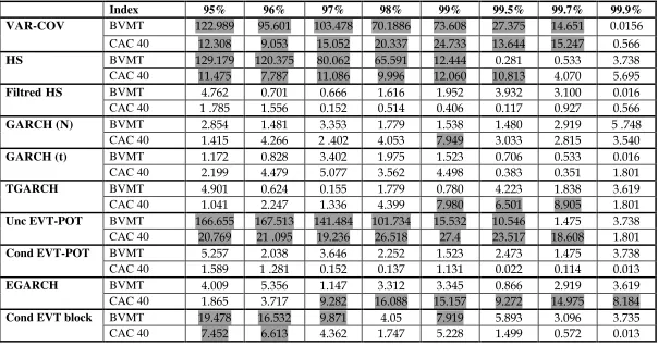
The relative out-of-sample performance for each model in term of violation ratio for the left tail (losses) at the window size of 1000 observations is calculated and presented in table 5 for BVMT index and in table 6 for the CAC 40 index. The number in parentheses are the ranking between ten competing models for each quantile. The violation ratio is defined as the number of times where the realized return is greater than estimated return (number of violation) divided by the total number of forecasts. An accurate and correct model is obtained when the expected
violation ratio is equal to . At qth quantile, the model predictions are expected to underpredict
the realized return = (1-q) percent of the time. A high violation ratio at qth quantile greater
than implies that the model excessively underepredicts the realized return. In the case of a
violation ratio less than , there is excessive overprediction of the realized return by the
underlying model. For instance, at the 0.95th quantile, the realized BVMT return is 4.711% of
0.01 0.02 0.03 0.04
0
1
2
3
4
5
Ordered Data
E
x
p
o
n
e
n
ti
a
l
Q
u
a
n
ti
le
s
0.015 0.020 0.025 0.030 0.035 0.040
0
1
2
3
4
5
Ordered Data
E
x
p
o
n
e
n
ti
a
l
Q
u
a
n
ti
le
s
Fig. 9 : QQ plots with exponential references distribution for the BVMT negatives returns
and the CAC 40 negatives returns over the threshold u
0.005 0.010 0.050
0
.0
0
.2
0
.4
0
.6
0
.8
1
.0
x (on log scale)
F
u
(x
-u
)
[image:21.595.158.439.108.289.2]
Fig.10: Fit of the estimated Generalized Pareto function for the BVMT ( in the left) and CAC 40 (in the right)
A violation ratio excessively greater than the expected ratio implies that the model signals less capital allocation and the portfolio risk is not properly hedged. In this case, the model will increase the risk exposure by underestimating it. A excessively lower violation ratio implies that the model signals a capital allocation more than necessary. In this case, the portfolio holder
allocates more to liquidity and registers an interest rate loss8.
For BVMT index, the Var-cov, unconditional EVT, HS and conditional block maxima EVT
methods are again the worst models for quantiles lower than the 0.99th quantile. AR-GARCH
models and filtred historical simulation provide the most performance for these quantiles.
Historical simulation provides the best results for quantiles higher than 0.98th except the 0.999th
8
Gençay, Selçuk, Ulugulyagci (2003), High volatility, thick tails and extreme value theory, Insurance: Mathematics and Economics.33 337 356.
0.005 0.010 0.050
0
.0
0
.2
0
.4
0
.6
0
.8
1
.0
x (on log scale)
F
u
(x
-u
quantile where Var-cov, filtred historical simulation and GARCH(t) perform best. This is the only quantile in which var-cov method not significantly overestimates nor underestimates the risk. Three VaR estimation methods give violation ratio that is statistically not overestimate nor underestimate risk at 95% level and for all quantiles: GARCH(t), EGARCH and conditional POT- EVT method.
At the 0.97th and 0.98th quantiles, TGARCH model performs the best with a violation ratio
of 3.105% and 2.088% respectively. It is followed by normal GARCH model and filtred
historical simulation. At 0.997th quantile, both historical simulation and GARCH(t) provide the
best violation ratio of 0.214% which amounts to 0.086% over-rejection. Conditional and unconditional POT EVT methods rank third with a ratio of 0.161% (0.139% over-rejection). The worst ratio is given by Var-cov, EGARCH and GARCH (N) models.
The GARCH(t) model provide the best performance at 0.95th , 0.997th , 0.999th quantiles, it
ranks second at 0.995th and fourth at the other remainder quantiles. Both conditional EVT
methods overestimate realized returns at all quantiles while the unconditional EVT
underestimates risk at all quantile except at 0.997th and 0.999th quantiles. We can conclude that
conditional POT- EVT method should be placed at the middle of the performance ranking between ten competing models while both conditional block EVT and unconditional EVT should be placed at the bottom.
For CAC 40 index, the conditional POT-EVT method provides the best violation ratio for
all quantiles except at 0.95th and at 0.99th quantile where it is placed at the second rank. The
second best model is filtred Historical Simulation which provide also an excellent performance
essentially at 0.97th , 0.99th and 0.995th quantiles. At 0.95th quantile, Historical Simulation
provides the best performance but its performance deteriorates at higher quantiles. It is followed by the conditional POT-EVT method and filtred historical simulation that ranks third.
At 0.999th quantile, conditional EVT methods provide the best results. The performance of
conditional block maxima at 0.98th, 0.995th and 0.997th quantiles is not bad but deteriorates at
lower quantiles less than 0.995th except the 0.98th quantile.
Three VaR estimation methods give violation ratio that is statistically not overestimate nor underestimate risk at 95% level and for all quantiles: GARCH(t), Filtred Historical Simulation and conditional POT- EVT method. The unconditional EVT, var- cov and all GARCH models underestimate risk at all quantiles.
In table 7, we present the Likelihood ratio tests statistics for the conditional LRcc for the ten
methods implemented and at eight differents significance levels. Our goal is to checks whether the probability of an exception occurring in one day is independent on events occurred in the day before. We reconfirm for both indices the previous results in tables 5 and 6 where Var-Cov and unconditional POT-EVT methods are not appropriate risk management techniques, as
for the majority of cases, LRcc statistics are significant (p-value<5%). Conditional POT- EVT
and filtred Historical Simulation methods are the best performers along with GARCH-t method. The GARCH models for the BVMT index have also recorded a similar success. Conditional Block Maxima method for the CAC 40 index produce acceptable VaR forecasts at high confidence.
While Historical Simulation method gives VaR violation ratios that are not significant most of time and for both indices and provides sometimes and at some quantiles the best results in
the base of conditional coverage criterion, it offers LRcc statistics that are significant.
Table 3
VaR(%) estimates-in absolute values- for the BVMT index on July 24,1998 and on December 30, 2005 and their mean for the out-sample period.
Model VaR ( % ) 95% 96% 97% 98% 99% 99.5% 99.7% 99.9%
In sample 30/12/2005
Var-Cov
Mean In sample 30/12/2005
HS
Mean In sample 30/12/2005
Filtred HS
Mean In sample 30/12/2005
GARCH (N)
Mean In sample 30/12/2005
GARCH (t)
Mean In sample 30/12/2005
TGARCH
Mean In sample 30/12/2005
Unc EVT POT
Mean In sample 30/12/2005
Cond EVT POT
Mean In sample 30/12/2005
EGARCH
Mean
In sample 0.528 0.567 0.618 0.689 0.808 0.926 1.011 1.192
30/12/2005 0.733 0.779 0.836 0.917 1.048 1.174 1.263 1.444 Cond EVT
Block
Table 4
VaR(%) estimates-in absolute values- for the CAC 40 index on Aout 4,1998 and on December 30, 2005 and their mean for the out-sample period.
Model VaR ( % ) 95% 96% 97% 98% 99% 99.5% 99.7% 99.9%
In sample 30/12/2005
Var-Cov
Mean In sample 30/12/2005
HS
Mean In sample 30/12/2005
Filtred HS
Mean In sample 30/12/2005
GARCH (N)
Mean In sample 30/12/2005
GARCH (t)
Mean In sample 30/12/2005
TGARCH
Mean In sample 30/12/2005
Unc EVT POT
Mean In sample 30/12/2005
Cond EVT POT
Mean In sample 30/12/2005
EGARCH
Mean
Table 5
VaR violation ratios for the left tail (losses) of daily BVMT returns ( in %)
Model 95% 96% 97% 98% 99% 99.5% 99.7% 99.9%
VAR-COV HS Filtred HS GARCH(N)
GARCH(t) TGARCH Unc EVT-POT Cond EVT POT
EGARCH Cond EVT block
The numbers in parentheses are the ranking between ten competing models for each quantile. Shaded number indicate statistically significant overestimation or underestimation of risk at 95% level.
Table 6
VaR violation ratios for the left tail (losses) of daily CAC 40 returns ( in %)
Model 95% 96% 97% 98% 99% 99.5% 99.7% 99.9%
VAR-COV HS
Filtred HS GARCH(N) GARCH(t) TGARCH Unc-EVT Cond-EVT EGARCH
Cond EVT block 3.757 (9) 2.910 (9) 2.222 (7) 1.640 (3) 0.529 (4) 0.317 (4) 0.217 (3) 0.106 (1)
The numbers in parentheses are the ranking between ten competing models for each quantile. Shaded number indicate statistically significant
Table 7
Likelihood ratio tests statistics for the conditional LRcc
Index 95% 96% 97% 98% 99% 99.5% 99.7% 99.9%
BVMT
VAR-COV
CAC 40 BVMT
HS
CAC 40 BVMT
Filtred HS
CAC 40 BVMT
GARCH (N)
CAC 40 BVMT
GARCH (t)
CAC 40 BVMT
TGARCH
CAC 40 BVMT
Unc EVT-POT
CAC 40 BVMT
Cond EVT-POT
CAC 40 BVMT
EGARCH
CAC 40 BVMT
Cond EVT block
CAC 40
[image:26.841.117.721.145.462.2]Q3 Q4 Q1 Q2 Q3 Q4 Q1 Q2 Q3 Q4 Q1 Q2 Q3 Q4 Q1 Q2 Q3 Q4 Q1 Q2 Q3 Q4 Q1 Q2 Q3 Q4 Q1 Q2 Q3 Q4 Q1
1998 1999 2000 2001 2002 2003 2004 2005 2006
-0
.0
3
-0
.0
2
-0
.0
1
0
.0
0
0
.0
1
0
.0
2
0
.0
3
0
.0
4
0
.0
5
loss GARCHt FHS Cond EVT
Q3 Q4 Q1 Q2 Q3 Q4 Q1 Q2 Q3 Q4 Q1 Q2 Q3 Q4 Q1 Q2 Q3 Q4 Q1 Q2 Q3 Q4 Q1 Q2 Q3 Q4 Q1 Q2 Q3 Q4 Q1
1998 1999 2000 2001 2002 2003 2004 2005 2006
-0
.0
2
0
.0
0
0
.0
2
0
.0
4
0
.0
6 loss
HS TGARCH Cond EVT
Q3 Q4 Q1 Q2 Q3 Q4 Q1 Q2 Q3 Q4 Q1 Q2 Q3 Q4 Q1 Q2 Q3 Q4 Q1 Q2 Q3 Q4 Q1 Q2 Q3 Q4 Q1 Q2 Q3 Q4 Q1
1998 1999 2000 2001 2002 2003 2004 2005 2006
-0
.0
2
0
.0
0
0
.0
2
0
.0
4
0
.0
6
0
.0
8
0
.1
0
[image:27.595.96.542.97.729.2]loss GARCHt UnEVT Block maxima
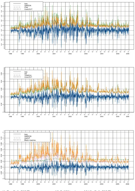
Fig. 11. Top: Daily BVMT negatives returns and VaR (95%) estimates. Middle: Daily BVMT negatives
Q4 Q1 Q2 Q3 Q4 Q1 Q2 Q3 Q4 Q1 Q2 Q3 Q4 Q1 Q2 Q3 Q4 Q1 Q2 Q3 Q4 Q1 Q2 Q3 Q4 Q1 Q2 Q3 Q4 Q1
1998 1999 2000 2001 2002 2003 2004 2005 2006
-0
.0
6
-0
.0
4
-0
.0
2
0
.0
0
0
.0
2
0
.0
4
0
.0
6
0
.0
8
0
.1
0
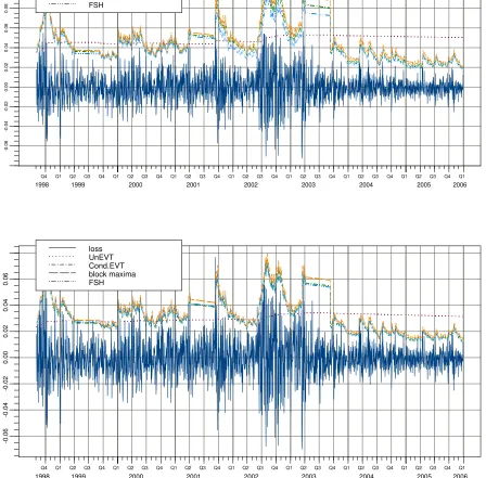
loss UnEVT Cond.EVT block maxima FSH
Q4 Q1 Q2 Q3 Q4 Q1 Q2 Q3 Q4 Q1 Q2 Q3 Q4 Q1 Q2 Q3 Q4 Q1 Q2 Q3 Q4 Q1 Q2 Q3 Q4 Q1 Q2 Q3 Q4 Q1
1998 1999 2000 2001 2002 2003 2004 2005 2006
-0
.0
6
-0
.0
4
-0
.0
2
0
.0
0
0
.0
2
0
.0
4
0
.0
6
[image:28.595.99.539.102.326.2]loss UnEVT Cond.EVT block maxima FSH
Fig. 12: Top: DailyCAC 40 negatives returns and VaR (99.7%) estimates.
Bottom: DailyCAC 40 negatives returns and VaR (98%) estimates
[image:28.595.95.543.138.579.2]set of extreme observations and as a result the unconditional VaR estimates are almost time independent. Unconditional EVT models are more suitable for long run forecasts of the extreme losses rather than being a day-to-day tool to measure the market risk.
For GARCH models and conditional EVT methods, variances are forecasted by an exponential model with declining weights on past observations and therefore are crucially dependent on the last few observations that is added in the sample. Conditional VaR forecasts increase with increasing volatility but also decrease with decreasing volatility indicate that conditional VaR estimates correspond more closely to the actual returns than the unconditional VaR estimates.
5. Conclusion
The purpose of this paper has been to attempt a comparative study of the predictive ability of VaR estimates from various estimation techniques. The main emphasis has been given to the Extreme Value methodology and to evaluate how well EVT- models perform in modelling the tails of distributions and in estimating and forecasting VaR measures.
Two different stock indexes, the BVMT and the CAC 40, have been investigated, and some differences between the indexes have been pointed at. Empirical results show that Var-Cov and unconditional POT-EVT methods are not appropriate risk management techniques for majority cases. Conditional POT- EVT and filtred Historical Simulation methods are the best performers along with GARCH-t method. The GARCH models for the BVMT index have also recorded a similar success. The conditional Block Maxima method for the CAC 40 index and at high confidence level produce acceptable VaR forecasts. GARCH models and conditional EVT offer high volatile quantile forecasts, while Historical simulation and unconditional EVT methods provide stable quantile forecasts. These two methods do not update the VaR number quickly when market volatility increases: when VaR violation occurs this day,the probability to observe an exceedence the next day is high. Hence, we observe clustered violations;
There are possible directions for future research. Methods presented and studied above are well-suited for providing forecasts of portfolio level risk measures such as the aggregate VaR. However they are less well-suited for providing input into the active portfolio and risk management process. A multivariate approach should be adopted to have a complete picture of the risk and to know the optimal portfolio weights to minimize portfolio variance. Multivariate models provide a forecast for the entire covariance matrix and are also better suited for calculating sensitivity risk measures. We can compute VaR variation when we add additional shares to my portfolio. Variety of multivariate volatility models can be used such as symmetric and asymmetric MGARCH and DCC models, Flexible multivariate GARCH introduced by Ledoit, Santa-Clara and Wolf (2003). Multivariate Extreme Value Theory offers also a tool for exploring cross-asset tail dependencies, which are not captured by standard correlation measures. Modelling the dependence structure of multivariate financial data using copulas is an approach recently rediscovered by a number of authors. The copula function provides a complete description of the association and the co-dependence proprieties of random variables at each point of a distribution.
References
Andersen, T.G. and T. Bollerslev (1998), Answering the Skeptics: Yes, Standard Volatility
Models Do Provide Accurate Forecasts International Economic Review 39, 885-905.