Numerical Simulation and Prediction of Groundwater Flow in a Coastal Aquifer of Southern India

http://dx.doi.org/10.4236/jwarp.2015.717122

How to cite this paper: Sathish, S. and Elango, L. (2015) Numerical Simulation and Prediction of Groundwater Flow in a Coastal Aquifer of Southern India. Journal of Water Resource and Protection, 7, 1483-1494.

http://dx.doi.org/10.4236/jwarp.2015.717122

Numerical Simulation and Prediction of

Groundwater Flow in a Coastal Aquifer of

Southern India

S. Sathish

, L. Elango

1_{Department of Geology, Anna University, Chennai, India}

2_{Present Address:Department of Geology, Adigrat University, Adigrat, Ethiopia}

Received 7 October 2015; accepted 22 December 2015; published 25 December 2015

Copyright © 2015 by authors and Scientific Research Publishing Inc.

This work is licensed under the Creative Commons Attribution International License (CC BY). http://creativecommons.org/licenses/by/4.0/

Abstract

Chennai is one of the most water-stressed cities in south India due to rapid industrialization and urbanization. The well fields located in north and south of the Chennai city meet part of the city’s water requirement. The south Chennai aquifer is surrounded by saline surface water on all sides. Since 1990, the influence of seawater in to this freshwater aquifer has been reported as an issue for consideration and mitigation measures. Therefore, in the present study an attempt is made to comprehend the status of aquifer with present level of pumping/recharge and to predict the be-havior with different hydrologic stresses. Numerical modeling was carried out by finite element approach using FEFLOW software. The model has been developed with three subsurface layers and simulation was processed from January 1998 to December 2020. The groundwater usage had varied from 11.3 MLD to 17.2 MLD during the period of study. If the recharge and discharge con-tinue in a similar pattern, the maximum level of freshwater decline will be 0.32 m at the end of 2020. Hence, prediction of behavior of this aquifer for increased discharge and decreased re-charge scenario has been carried out. It is found that with an increase of disre-charge, there is a sharp change in interface of seawater and freshwater. This model can be used as a tool to under-stand the aquifer regionally and to plan proper groundwater management measures.

Keywords

Coastal Aquifer, Seawater Intrusion, Groundwater Modeling, Chennai

1. Introduction

Groundwater quality depends on land use practice, climatic conditions and pollution free sources among several

groundwater supply and faces seawater intrusion problem since 1990’s. In this context, state authorities reduced pumping to 3.4 MLD from maximum of 9 MLD [5]. In order to understand the behavior of coastal aquifer sys-tem in South Chennai, various studies have been carried out with respect to quality of groundwater, fluctuation of groundwater level etc. by [6]-[11]. The authors [12] identified the recharge characteristics and pumping pat-tern of the aquifer by groundwater modeling. However, due to increased land use changes (from scrubland/open land to residential sparse) and climatic variability, it is necessary to predict the long term behavior of aquifer to various hydrological stresses. Hence, a study has been carried out in South Chennai aquifer, with reference to change in recharge and discharge characteristics. The results obtained from this work may assist for the sustain-able developments and to take precaution measures.

2. Materials and Methodology

2.1. Study Area

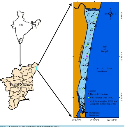
The geographic location of the present study area is tropical wet and dry zone from longitude of 80˚14'5.698"E to 80˚16'37.251"E and from latitude of 80˚14'5.698"N to 80˚14'5.698"N. The total study area is 35 sq. km, which is surrounded by saline surface water on all four sides (Figure 1). It is bounded by the Adyar River in North, the Muttukadu estuary in south, the Bay of Bengal in east and the Buckingham canal in the West. The maximum elevation is 12 m above MSL towards the north and the minimum is 0 MSL. The central part of the area is elevated along N-S stretch with gentle slope towards east and west. The ground slope varies from 0.61% to 10.42% and holds groundwater table as mound. The geomorphologic features are controlled by erosion and depositional regimes. The landforms comprise of terraces, different levels of rising tract of surface due to tidal effect, oscillation in sea level and action of wind which forms a series of levels with gentle slope on both the sides. The aquifer comprises of coastal alluvial deposits of Quaternary and Recent unconsolidated sediments and followed by charnockites of Archean age. The unconsolidated sediments comprises of medium, fine and coarse sand, clay, sandy clay, clayey sand, gravels and pebbles.

The western part of the study area which is bounded by the Buckingham canal is dominated by clay and sandy clay, whereas the eastern part is dominated by sand of various sizes [9][10]. The Adyar River carries flow throughout the year with an average of 89.43 Million Cubic Meter per Year [13]. The quality of water in Adyar River is not suitable for any purpose due to mixing of domestic and industrial effluents. The Buckingham Canal (western boundary) which was originally established for navigation is presently not in use [14]. Both Adyar River and Buckingham canal serves as flood moderators especially during the monsoon (wet) period. Muttukadu estuary in the south also has saline water with high organic content [15].

2.2. Data Collection and Model Development

Figure 1. Location of the study area and monitoring wells.

every three months. The groundwater level was measured using groundwater level indicator. The minimum and maximum depths of the investigated wells are 3 m and 18.43 m respectively. All the investigated wells penetrate the unconsolidated formation (sand, sandy clay and clayey sand). Based on the problem, code selection has been made to comprehend the aquifer status. Hence, to consider an accurate boundary along water body, to get sound approximation and quality, finite element approach [17] was utilized using FEFLOW-FMH3D software. FEFLOW is a version of the modular finite element simulation system for modeling 2D and 3D flow, mass and heat transport. It is capable of considering both saturated and unsaturated conditions. The pre- and post-proces- sor was handled for graphical representation and analysis of the output.

Figure 2. Conceptualization of the study area.

hydraulic conductivity and specific yield, were assigned to each layer. Due to the presence of clay along the western boundary, large variation in the property of aquifer was observed. A specific yield of 0.05 was assigned along the western boundary where clay was present, 0.14 was assigned where clay was dominant with sand, 0.18 was assigned where sand was dominant with clay and 0.26 was assigned where sand was present. Hydraulic conductivity varied from 6 md−1 to 30 md−1. The aquifer is free of surface water bodies such as lake, pond etc., but bounded by surface water on all the sides. Hence rainfall is the main source of groundwater recharge. The recharge was used as per suggested range by previous publications. The groundwater discharge estimation for present condition was done using the measured data including groundwater level and aquifer parameter and from the simulated model results. During model prediction from June 2010 to December 2020, the recharge was assigned from past 10 years of monthly average rainfall.

The simulation was carried out from January 1998 to December 2020. The parameter estimation was done in steady state calibration with groundwater level in 19 well locations [12] (Figure 1). The estimated parameters from the steady state calibration were used as the initial condition for transient state calibration, which was car-ried out with time dependent recharge and discharge rates. The pumping of groundwater was assigned based on the previous report, land use and land cover pattern. Transient state calibration was done for 84 time steps from January 1998 to December 2004 in monthly interval. Validation has been carried out until from January 2005 to May 2010 and prediction was done till December 2020.

3. Result and Discussion

3.1. Hydrogeological Condition

The groundwater table is present under unconfined condition and it appears as mound and follows the trend of the topography. The maximum elevation of groundwater level was 5 m above MSL in the southern part of the area during February 2009 (Figure 3). This was due to high rainfall (867.2 mm of rainfall in NE monsoon) compared to the five set of monsoon in 2008-2010. The fluctuation of groundwater was analyzed from long term available groundwater level data of eight wells. The maximum range of groundwater level was recorded to 2.95 m. above MSL.

3.2. Present Condition of Seawater Influence

ex-plains the influence of them on the aquifer. The increase in EC downward depth is due to the effect of interac-tion with seawater (Well No. 35). The vertical variainterac-tion of EC in the wells located in middle stretch is under permissible limit. The comparison of EC in two hydrological cycles from 2008 to 2010 confirms that the influ-ence of seawater is maximum in the northern boundary. The distance of influinflu-ence of seawater is varying from wet to dry season, it is up to 1.4 km during end of dry season (August) and it is about 0.4 km in wet season (Figure 5).

Figure 3. Spatial variation of groundwater level (m msl).

Figure 5. Influence of seawater in various seasons.

3.3. Model Calibration

The values of aquifer parameters like hydraulic conductivity and specific yield were collected from literatures and adjusted up to ±10% to obtain more realistic aquifer parameters by comparing observed groundwater level. The horizontal hydraulic conductivity used for steady state calibration varies between 6 md−1 to 30 md−1. One tenth of horizontal hydraulic conductivity is used as vertical hydraulic conductivity. The specific yield value va-ries from 0.05 to 0.26. The steady state calibration was resulted with an accuracy of 0.8387 (Figure 6). The dif-ference between observed and computed groundwater levels varies from 0.2 m to 1.3 m. This variation might be due to local variations in topographical elevation over short distances.

The fluctuation of groundwater level obtained from the eight long term monitoring wells have been utilized for the purpose of transient state calibration. During transient state calibration, the estimated parameters from steady state calibration were modified within the permissible limit (±10%). Calibration of model in transient state flow condition was done by trial and error method and obtained good match between the computed and observed groundwater levels over space and time. The initial input values and the modified values of hydraulic conductivity and specific yield during calibration are presented in Table 1. During transient state calibration, the maximum difference between observed and calibrated groundwater level is 1.1 m and this is observed in well No.3 (Figure 7).

3.4. Groundwater Recharge and Discharge

Figure 6. Initial observed and calibrated groundwater levels.

Figure 7. Observed and calibrated groundwater level.

Table 1. Initial and calibrated hydraulic parameters.

S. No. Geology of the area

Hydraulic conductivity (md−1) Specific yield

Initial Calibrated Initial Calibrated

1 Layer-I 8 - 30 6 - 28 0.05 - 0.26 0.07 - 0.26

2 Layer-II 6 - 8 5 - 6 0.05 - 0.10 0.05 - 0.14

3 Layer-III 6 - 11 5 - 9 0.05 - 0.16 0.05 - 0.18

(June to September) and north east monsoon (October to December) are shown in Figure 8. The discharge of groundwater is usually higher in the transition period compared to the north east monsoon when the rainfall is high. The discharge of groundwater varied from around 9 MLD to 18 MLD from 1998 to 2007. During the pe-riod of study (August 2008 to May 2010) the groundwater discharge varied from 11.3 MLD to 17.2 MLD.

3.5. Validation

The validation of groundwater level was carried out for 65 stress periods in monthly intervals from January 2005 to May 2010. The temporal variation of observed and computed groundwater level for the period of validation until December 2007 is shown in Figure 7. The continuation of validation of groundwater level until May 2010 was done with groundwater level measurement during the period of study (Figure 9). The spatial variation of observed and validated level is shown in Figure 10.

3.6. Prediction

Figure 8. Estimated groundwater discharge in the study area.

Figure 9. Observed and computed groundwater level during validation.

due to monsoon failure causes groundwater level decline. Recently, the failure of seasonal rainfall has forced the aquifer into critical condition. To understand the behavior of this aquifer in near future the model was run with present level of pumping and recharge rate and in various scenarios of different hydrological stresses such as in-creasing and dein-creasing the pumping and recharge rate respectively.

3.6.1. Prediction with Present Scenario

After validating the groundwater model, the model was run for a period of 126 months (10 1/2 years) from June 2010 to December 2020 in monthly interval. The pumping rate of 11.3 MLD to 17.2 MLD was used for predic-tion, which is the pumping rate obtained from model during the period of August 2008 to May 2010. The long term annual average rainfall is 1066 mm, which is calculated based on rain-gauge measurements obtained over the past 10 years and has been used previously in the model. The recharge rate varies from 0.46 mmd−1 to 47.49 mmd−1. Based on this scenario, the spatial and temporal variation graph indicates that the groundwater level va-ries from 0.114 m to 4.26 m during the period from June 2010 to December 2020. The minimum level of groundwater (0.114 m) is observed in well No. 35 (Figure 11) which is located near the coastal boundary. The maximum groundwater level (4.26 m) is observed in well No. 25 which is located at the central stretch of the study area.

Figure 10. Spatial variation of observed and validated groundwater level.

cline of groundwater level occurs up to 0.60 m at the end of the model period (2020). The decline of groundwa-ter is high in well No. 32 which is located in the northern part of the area. The decline is also high in well No. 26 and 29 which are located at the elevated groundwater level area. Along the coastal region, the decline in groundwater level is very less as (0.014 m) occurred in well No. 35. In the scenario with 10% increase in dis-charge, the discharge rate has increased as 12.4 MLD to 18.9 MLD from the present discharge rate (11.3 MLD to 17.2 MLD). The results indicate that the decline of groundwater level occurred up to 1m at the end of year 2020. Similar to the results of decline of groundwater level in 5% increased scenario, the decline of groundwater level is high in well No. 32, 26 and 29. Along the coastal region, the decline of groundwater level is compara-tively less (about 0.17 m).

In the prediction with 5% reduced recharge rate, it was observed that the groundwater level declined by maximum of 0.726 m in well No. 29 which is located in the northern part. The decline is high in the northern part compared to overall fluctuation of groundwater level. In well No. 35 which is located very near to the coast shows 0.091 decline in groundwater level. The groundwater level fluctuation varies from 0.301 m to 1.692 m during the study period. The minimum fluctuation is comparatively higher than fluctuation under present predic-tion (0.278 m) and the maximum fluctuapredic-tion is comparatively lesser than fluctuapredic-tion under present predicpredic-tion (2.04 m). The groundwater level fluctuation is high in the northern part of the area. The fluctuation is compara-tively less than the annual average fluctuation in this aquifer.

Similarly, in the prediction with 10% reduced recharge rate, the groundwater level decline is up to 1.52 m in well No. 29. The well located near the coastal surface shows 0.171 m decline in the groundwater level. The groundwater level fluctuation is from 0.295 m to 1.697 m. It is also comparatively lesser than the fluctuation of groundwater level in this aquifer under the present scenario prediction. The negative groundwater level was no-ticed from end of July 2014 (Figure 12). By comparing the results obtained from the entire scenario, it was no-ticed that the northern part of the area is more sensitive to recharge and discharge condition. Urbanization plays a major role in controlling the groundwater level fluctuation and the seawater intrusion into the aquifer.

Table 2. Groundwater level under various hydrological stress at the end of 2020.

Scenario

Groundwater level (m) Fluctuation (m) Discharge MLD Recharge (mm/d)

Yearly Rainfall (mm)

Min Max Min Max Min Max Min Max

+5% recharge 0.169 3.837 0.314 2.03 11.3 17.2 0.483 49.865 1119

+10% recharge 0.352 4.536 0.223 2.25 11.3 17.2 0.506 52.24 1172

+5% discharge 0.101 3.74 0.278 2.20 11.4 18.1 0.46 47.49 1066

+10% discharge 0.089 3.41 0.278 1.30 12.4 18.9 0.46 47.49 1066

−5% recharge 0.059 2.43 0.301 1.69 11.3 17.2 0.437 45.115 1012

−10% recharge 0.009 1.70 0.212 1.48 11.3 17.2 0.414 42.74 959

−5% discharge 0.148 3.78 0.262 1.22 10.7 16.3 0.46 47.49 1066

Figure 12. Prediction with reduced recharge rate.

4. Conclusion

Numerical simulation and prediction of groundwater level in coastal aquifer of South Chennai in India, has been carried out. The hydrologic condition of the study area of groundwater abstraction is high in dry period and low during the period of north east monsoon when rainfall is high. The abstraction of groundwater varied from 8.7 MLD to 18.1 MLD from 1998 to 2007. However, from August 2008 to May 2010 the groundwater discharge varied from 11.3 MLD to 17.2 MLD. It indicates that the discharge rate is comparatively less than the recent past. But still if the recharge and discharge continues in the same trend the maximum decline in groundwater level will be 0.32m at the end of 2020. The maximum of reduction in aquifer storage of groundwater is up to 1,019,200 m3, it may further increase seawater intrusion up to 12 m in to the land. Comparison of land use and land cover map from 2004 to 2012 indicates the rise in settlements which may impose high pumping rate. In-crease in discharge by 5% results to a maximum decline of groundwater level by 0.60 m with maximum inIn-crease of seawater intrusion up to 25 m in land at the end of the year 2020. Increase in discharge by 10%, the ground-water level will decline up to 1 m. If the recharge rate is lowered by 10% from the normal suggested rainfall re-charge range, the groundwater level lowers below the sea level. Thus the model was used to understand the ex-pected changes in groundwater level under different hydrological stresses.

Acknowledgements

ble Water Supply in India. DSDS Special Event Water: Out Global Common, New Delhi.

[5] Gnanasundar, D. (2001) Hydrogeochemical Studies and Regional Flow Modeling of South Chennai Sandy Aquifer. Dissertation, Anna University, Chennai—600 025.

[6] Annapoorani, A., Murugesan, A., Ramu, A. and Renganathan, N.G. (2013) Groundwater Quality Assessment in Coast-al Regions of Chennai City, Tamil Nadu, India—Case Study. International Journal of Recent Scientific Research, 4, 171-176.

[7] Elango, L., Ramachandran, S. and Chowdary, Y.S.N. (1992) Groundwater Quality in Coastal Regions of South Madras. Indian Journal of Environmental Health, 34, 318-325.

[8] Palanivelu, K., Nisha Priya, M., Muthamil Selvan, A. and Natesan, U. (2006) Water Quality Assessment in the Tsuna-mi-Affected Coastal Areas of Chennai. Current Science, 91, 583-584.

[9] Sathish, S., Elango, L., Rajesh, R. and Sarma, V.S. (2011) Application of Three Dimensional Electrical Resistivity Tomography to Identify Seawater Intrusion. Earth Science India, 4, 21-28.

[10] Sathish, S., Elango, L., Rajesh, R. and Sarma, V.S. (2011) Assessment of Seawater Mixing in a Coastal Aquifer by High Resolution Electrical Resistivity Tomography. International Journal of Environmental Science & Technology, 8, 483-492. http://dx.doi.org/10.1007/BF03326234

[11] Sathish, S. and Elango, L. (2011) Groundwater Quality and Vulnerability Mapping of an Unconfined Coastal Aquifer. Journal of Spatial Hydrology, 11, 18-33.

[12] Gnanasundar, D. and Elango, L. (2000) Groundwater Flow Modeling of a Coastal Aquifer near Chennai City, India. Journal of Indian Water Resources Society, 20, 162-164.

[13] CGWB (2008) District Groundwater Brouchure, Chennai District, Tamil Nadu. 1-15.

[14] Packialakshmi, S. and Ambujam, N.K. (2012) A Hydrochemical and Geological Investigation on the Mambakkam Mini Watershed, Kancheepuram District, Tamil Nadu. Environmental Monitoring and Assessment, 184, 3293-3306.

http://dx.doi.org/10.1007/s10661-011-2189-1

[15] Gangabaheerathi, C. and Revathi, K. (2013) Bacterial Contaminants in Crassostrea Madrasensis Harvested from Mut-tukadu Backwaters. Indian Journal of Applied & Pure Biology, 28, 91-94.

[16] Senthilkumar, M., Gnanasundar, D. and Elango, L. (2001) Geophysical Studies to Determine Hydraulic Characteristics of an Alluvial Aquifer. Journal of Environmental Hydrology, 9, 1-8.