Choosing the extent of private participation in public services: A computable general equilibrium perspective

Munich Personal RePEc Archive

Choosing the extent of private

participation in public services: A

computable general equilibrium

perspective

Chisari, Omar O. and Lambardi, Germán D. and Romero,

Carlos A.

Centro de Estudios Económicos de la Regulación - Universidad

Argentina de la Empresa

September 2007

Online at

https://mpra.ub.uni-muenchen.de/15358/

Choosing the extent of private participation in public services:

A computable general equilibrium perspective

Omar O. Chisari

Instituto de Economía – Universidad Argentina de la Empresa

Germán D. Lambardi

Universidad de Toulouse

Carlos A. Romero

Centro de Estudios Económicos de la Regulación – Universidad Argentina de la Empresa

Abstract:

What determines the propensity to reduce or widen the extent of public ownership? Why has there been a

tendency to privatise and concede public utilities during the nineties? The answers to these questions

depend both on macroeconomic and microeconomic considerations. And correct answers could also help

to avoid or prevent inefficient reversals and frustrations that jeopardize reform processes. An alternative

perspective, that combines micro and macro arguments, is given by general equilibrium models. The

objective of this paper is to explore the rationality of the decision of choosing the implicit “technologies”

of private and public operators of utilities in an economy that has fiscal budget and trade balance in

equilibrium. The simulations confirm that the choice of the technology to be used for servicing

infrastructure depends on deep parameters of efficiency and costs. The model shows that there are

plausible scenarios where the selection is not unique.

Choosing the extent of private participation in public services: a

computable general equilibrium perspective

1. Introduction.

What determines the propensity to reduce or widen the extent of public

ownership? Why has there been a tendency to privatise and concede public utilities

during the nineties?

The answers to these questions depend both on macroeconomic and

microeconomic considerations. And correct answers could also help to avoid or prevent

inefficient reversals and frustrations that jeopardize reform processes.

On the microeconomic side, there are two prominent theories1. One, emphasizes the role of public ownership to resolve contractual problems and to influence the

decisions of the firms in certain sensitive issues for the politicians; it is easier to control

the decisions of the firm (on employment levels, for example) when the company is

under public ownership. The other focuses on the self exclusion of private sector under

government opportunism; if taxes and regulations are too unstable and endogenous, risk

of arbitrariness discourages private investments, and public ownership is the only

possibility.

Macro considerations have been concentrated in the need of controlling public

deficits, obtaining revenues from privatisations and concessions, fostering growth

through efficiency enhancements and obtaining price reductions via competitive

environments.

One additional point to consider is the all-or-nothing character of the choice.

That is, are there gains of having private operators coexisting and competing with a

public enterprise?

There are two aspects to take into account:

1) Efficiency gains given the reciprocal benchmarking, though in this case it is

difficult to say why not benchmarking private operators and why a mix

public/private is better.

2) Gains due to harder competition, though a similar observation applies and

competition could prevail between private operators. In fact, having only private

operators could alleviate potential problems of moral hazard of public sector

being involved simultaneously in operation and regulation.

2. The general equilibrium approach.

An alternative perspective, that combines micro and macro arguments, is given

by general equilibrium models. This perspective has not been fully explored, and there

are only a few examples –e.g. Chisari, Estache and Romero (1999). Beyond short term

increases in revenue for the governments, efficiency gains for the economy could justify

higher presence of private sector.

General equilibrium gives a framework of consistency that impedes counting

gains more than once, obliges to represent budget constraints of all agents –including

transfers- and gives net welfare results after taking into account changes in relative

prices and factor rewards. In fact, changes in factor rewards could change expected

gains of privatisations and government activity…or not. And it is in the last case when

arguments in favour of private operation are stronger.

In this paper the objective is to explore the rationality of the decision of

choosing the implicit “technologies” of private and public operators of utilities in an

economy that has fiscal budget and trade balance in equilibrium.

We do not consider neither asymmetries of information nor political

opportunism. They are certainly important elements to take into account, but it seems to

be also relevant to focus on the core of the workings of the economy. What happens

with relative prices and factor rewards after the privatisation or concession, net welfares

gains and their distribution –even or not- the sensitivity of the decision to changes in

fundamental parameters, like the cost of capital, deserve deeper examination.

In broad terms, we will assume that the extreme cases of public and private

 Public enterprises show lower efficiency levels in the use of intermediate inputs

and employment.

 This inefficiency implies that public enterprises must be subsidized, and therefore, that taxes or prices of utilities services must be higher.

 This inefficiency is also present in the investment process: one unit of investment produces more units of capital installed under private operation (or

less units of investments are needed to compose one unit of capital).

 However the share of imported intermediate inputs is higher in the case of private operators, since new investments and methods are complementary of

inputs and services provided by the rest of the world.

 Capital reward of private operators in determined basically by its cost of opportunity in the rest of the world.

Given these elements, the typical choice will involve:

 Taking into account that evidence tends to confirm that under public hands inefficiencies are higher, that more resources will be necessary to operate

utilities diverting them from other (valuable) activities, and that subsidies will

have to be covered with taxes or higher prices and that this creates further

inefficiencies in the allocation of resources.

 Realizing that though private operators are more efficient, productivity of capital in the rest of the world becomes a relevant benchmark as the minimum required

reward for private capital, and that potential transfer of dividends abroad could

put pressure on trade balance. The economy will enjoy higher efficiency and

performance standards, but at the cost of having to devote more resources to

export markets.

So the basic comparison can be reduced to the minimum cost choice between

contributing to exports with local effort and consumption sacrifice or accepting

inefficiencies and costs of misallocation of resources due to subsidisation. The intention

is trying to give general equilibrium hints to the answers posed at the beginning of this

paper and to consider thresholds for the cost of capital and public funds full costs that

There are some provisos to take into consideration. The results must be

examined both under full employment and unemployment; in the last case, the results

will depend on the rule of indexation of wages. Under unemployment, efficiency gains

will be more important for obtaining increases in scales of operation that will influence

positively welfare.

Asymmetries of information are not part of the model. It is true that they a

cornerstone of regulatory economics, but at this stages the differences of dealing with

them under public or private operation will only add confusion to the results. In fact,

especially under high-powered regimes, the capacity and willingness to deal with

asymmetries of information will be probably higher under private hands and that would

be a reason for recommending private ownership or operation. But, what of the costs?

3. Basic analytical structure.

The analysis is based on a standard CGE model with regulation and service

obligations (see Box 1). So the economy must choose between: 1) a local technology

provided by the public enterprises, or 2) an updated –probably capital intensive-

technology that uses mobile capital.

A fundamental difference of these technologies is that while capital is

considered a sunk cost for public enterprises, it is not for private operators, though these

conditions can be relaxed. The idea is to compare the on going model –the public

enterprises technology- with a new one, more demanding in terms of capital

BOX 1: Regulatory Regimes and Service Obligations in a CGE

Service obligation is interpreted as the passive adjustment of services supply to demand in the regulated sector. This assumption prevents need to rely on rationing which is quite realistic in the context of modern infrastructure reforms. If this assumption were not included, we would need to accept some form of rationing of customers (households or firms), and this will make any model much more complicated and ad-hoc.

Most regulatory regimes establish explicitly this obligation in the contract, and its violation has not only direct economic costs but also hinders on the reputation of the firm. Service obligation increases costs to the firm (real and expected) and is compensated with the tariff and, very often, with the commitment by the regulator of protecting incumbents by legally blocking the entry of new competitors. A temporary “no entry” condition is, in fact, a second important characteristics of modern infrastructure reforms, which guarantees a return on assets, when perceived commercial risk levels could be aggravated by the concern for entry and become a participation constraint for the private sector.

With the Service Obligation hypothesis, there are two possible cases. In the first case, there is enough installed capacity to cover the necessities of clients and the main issue is for the firm to get a subsidy to cover the difference between marginal cost and regulated price. In the second case, the capacity is insufficient and additional investment is needed. This second option (with constant marginal costs) is used exceptionally when demand becomes too high. For the first option, we assume that the subsidy is paid by the shareholders of the firm in the case of the price-cap regime. With this strategy, existence of equilibrium can be shown using the proofs already available for the standard general equilibrium models with taxes. The price-cap or the rate-of-return regulation can be interpreted as special mark-up rules that are in fact taxes for which the revenue accrues to (or is extracted from) the owners of the firms.

To simplify, it may be useful to complement the discussion with a graphic beginning with the model of alternative technology. In fact, Graph 1 shows the case of an alternative technology when demand (Da) is low enough as to have excess of installed capacity. PR and qR denote the tariff in terms of the numeraire and the

production level in the regulated sector, respectively. MC represents the marginal cost of the existing technology (the increasing segment) and an alternative technology (the constant marginal cost section of the curve), and 1/ stands for the benchmark regulated price.

Given Da, pR should fall to 0

R

p . However, a tax t is imposed (mark-up) to compensate owners of capital so that

1 *

(1 )

R R

p  t p = 1/.

“Tax” revenue is transferred from customers to shareholders of the regulated firm. This t could be negative as it is shown in Graph 2, that it is a subsidy s. If an alternative technology does not exist, the firm will continue operating if the additional units (A) marginal costs are covered (triangle S). Since the obligation of service was established in the original contract between the regulators and shareholders, we assume that the shareholders cover the excess of costs –implicitly in the form of a subsidy to the operative management of the firm. This internal subsidy s is depicted in the figure below; in this case s is computed so that net price to customers equals the price-cap settled at levelp_R.

In summary, Graph 2 shows the case of an internal subsidy, funded with a tax on the shareholders of the regulated firm. When shareholders are foreign, this subsidy will be accompanied by an inflow of capital that reduces the need of trade surplus. Graph 2 also illustrates the case when the firm has the alternative of importing international capital. The incremental cost of the new technology is given by w*A/µ, where w* is the foreign factor reward and µ its average productivity. The firm will compare this cost with S, to choose the method for servicing the market. However, this will have consequences on the current account; if the firm covers the deficit with the existing technology there will be an inflow of capital (though temporary); instead if the alternative technology is employed, the additional reward of foreign factors will impose a burden.

Graph 1: Non-operative price-cap

q R

1/µ

Da

t p R0

p R1

p R

Graph 2: Subsidy and alternative technology

q R

pR

D MC

MC(1-s)

S s

A

Source: Chisari, Estache, Lambardi y Romero (2003).

To simulate the model we will use a Social Accounting Matrix of reduced

dimensions that captures the main characteristics of a developing economy, in terms of

share of public services in GDP.

There is a basic structure that will be specialized to consider the public and

private technologies. For the sake of presentation, the public technology is discussed

first.

Each sector uses two different factors: one mobile, labor, and one non mobile,

specific capital2. There are four domestic sectors of production (activities): I={1,2,N,R}, two of them are tradable sectors, T={1,2}, and the rest are producers of goods and

2

services that are not tradable; sector N produces services and sector R represents sectors

under regulation.

Each activity produces only one commodity represented by J={1,2,N,R}. We

assume that the utility and production functions correspond to the traditional

neoclassical version. However, production sectors are related through input-output

transactions, which play an important role in understanding the net impact of regulation

on the economy. Prices of tradable goods are determined by the rest of the world3, and domestic agents also import consumption goods that are imperfect substitutes of local

production. In this version, it is assumed that imported goods are not used for

production.

The analytical representation of the aggregated regulated sector in this section

deserves more attention. Though it is natural to think that the production function of that

sector should exhibit some economies of scale or sub-additivity, we will assume that

there are not non-convexities once specific capital is installed. This is a simplification

with obvious theoretical costs, but it also contributes to concentrate our effort in

determining the impact of regulatory mechanisms and not on the properties of the

production set4. The public technology works with installed capital. The alternative technology gives some hints on the long run effects; in that case, we assume constant

returns to scale.

Domestic household.

We assume that there is an only domestic agent that makes the decision on the

consumption plan and receives all factor rewards (except for the regulated firm) and

profits. So, we will not be paying attention to personal income distribution matters,

though we can analyze factor distribution. This agent collects also all taxes and grants

subsidies. Net welfare of this household will therefore represent social welfare.

The domestic agent maximizes the utility function u c c c( ,1 2, N,c mR, )subject to:

3 _{The “small country assumption” in terms of Kehoe and Kehoe (1994).}

<1>   * / ( , ) R I

T T R R N N m I R R R

T I R

p c  p c  p c p mwL r K  tp G L K





where  is the share of domestic agents in profits of the regulated sector *

R

 and the last

term corresponds to the compensatory transfer from domestic customers ( t  0) or to

the firm from its shareholders (t  0). Under public ownership,  = 1. In both cases, under price cap, t is computed so that pR = 1/(1+t). From utility maximization, we

obtain the familiar first order conditions:

<2> ' ' T

c m T m

u u  p p

<3> u'_R u'_m p_R p_m

<4> u'_N u_m'  p_N p_m

cT is consumption of domestic tradable goods, cR is the consumption of goods and

services under regulation and m are imports (a good produced abroad but not

domestically) and pT, pR and pm are their respective prices. w is the wage rate and rI is

the rate of return on capital in each sector. L and Krepresent the domestic agent

endowments of labor and capital.

Domestic Production Sectors

F, H and G are the production function of the tradable, non-tradable and

regulated sectors, respectively. We assume constant returns to scales in all cases. As we

mentioned, this is a simplification that helps to avoid problems of existence of

equilibrium. However, in this version, once capital is sunk, it does not seem to be

unrealistic.

a. Tradable Sectors

There is one firm that maximizes profits in each tradable sector. The net price for the

firm is the price to consumers less the cost of intermediate inputs..

<5> _{T T J T, J R T, R N T, N T}( _T, _T) _{T T T}

J T T

p a p a p a p F L K wL r K

            





for every T=1,2. Notice that firms observe the incentive given by the net price after

intermediate inputs costs. The maximum profit conditions are:

<6> _{T J T, J R T, R N T, N L} J T

p a p a p a p F w



     

 

<7> _{T J T, J R T, R N T, N K T} J T

p a p a p a p F r



     

 





In both cases, the value of marginal product (corrected for intermediate costs) is

equalized to the reward of the factor. Notice that we are not assuming export or import

taxes but they can be introduced easily as ad valorem taxes.

b. Non-tradable Sector

Services and other non tradable goods are produced using labor and capital.

Capital is specialized and non mobile. Equation (8) corresponds to profits definition,

and equations (9) and (10) to optimization conditions:

<8> _{N N T N, T R N, R} ( _N, _N) _{N N N} T

p a p a p H L K wL r K

      

 





<9> N T N, T R N, R L T

p a p a p H w

    

 





<10> _{N T N, T R N, R N N} T

p a p a p H r

    

 





c. Public utilities or regulated sector

As we mentioned above, the regulated firm is treated as a neoclassical firm.

There is no entry and service obligations are established. Net price is obtained as the

difference between the regulated price and intermediate cost.

<11> _{R R T R, T N R, N} ( _R, _R) _R T

p a p a p G L K wL

     

 





Notice that in this expression KR is given. The total rate of return of this sector is

/

R R R

r  K . The optimal condition for profits is: <12> _{R T R, T N R, N L}

T

p a p b p G w

    

 





aR,T and aT,R are input-output coefficients used to represent also technical gains due to

privatization. A reduction in aT,R is an improvement of efficiency internal to the public

service firms, which reduces the requirement of intermediate inputs per unit of product.

aR,T is a reduction of the requirement of regulated input per unit of tradable output (due

Rest of the world.

a. Production sectors.

The rest of the world produces substitutes for our exports and import goods,

using a factor of production F. Equations (19) to (22) give an alternative technology

available for foreign owners to fulfill their obligation of services, using mobile capital.

<13> * ( ) * m pm Fm w Fm

   

<14> * ( ) * T pT T FT w FT

   

<15> p_m w*

<16> p_T_T w* <17> ms(F_m) <18> s ( )

T T

x  F

In the case of α’ and _T constants, international terms of trade will be given by

T m T

p p   (small economy assumption).

*

m

 and _T* represent profits in the rest of the world industries that produce

import goods and perfect substitutes of tradable goods. w*, the numeraire, is the wage

rate of the only factor used abroad.

Fm and FT are factor quantities employed in the corresponding industries. The

production functions: α(Fm) and βT(FT) give the total supply in equations <16>, <17>

and <18>.

b. Households

Consumers in the rest of the world receive the rents of foreign factors, including

capital installed in the regulated sector as well as profits in that sector. It maximizes a

utility function *

( _T, )

v x m that depends on the consumption of our tradable goods and of

<19> _m * _{T T} * (1 ) _{R m}* _T* _R ( _R, _R) T

p m p x w F    



Foreign agent receives profits and capital return of the regulated sector, as well as the

wage rate (cost of capital) F and the proceedings of the mark-up factor. XT are exports

that are domestic tradable goods bought by the foreign agent. The last term in equation

<19> stands for the endogenous mark-up (positive) or internal subsidy (negative)

computed as the difference between the benchmark tariff 1/ (as seen by customers) and

PR

Market equilibrium conditions

Equations (20) to (27) represent the equilibrium conditions for factors used

domestically, and (28) is the equilibrium condition for the foreign factor. Equations (25)

to (27) correspond to equilibrium in markets for goods: regulated, non regulated and

imports.

<20> L L₁ L₂L_RL_N

<21> K_T K_T (T1, 2)

<22> K_N K_N

<23> _{m T} T

F F 



<24> ( _R, _R) _{R R T, T}( _T, _T) _{R N,} ( _N, _N) _R T

G L K q 



<25> ( , ) s _, ( , ) _, ( , )

T T T T T R R R T N N N T T

F L K x a G L K a H L K c x

<26> ( N, N) N T_, T( T, T) N R_, ( R, R) N T

H L K 



<27> ms m m*

Trade balance

We can now see how the relation between the mark-up factor (and its mechanism

of adjustment) and the trade balance arises in the model. From <1>:

/{ } /{ }

* I ( , )

R R I I I R R R R

I R I R

p c 





/{ } /{ }

( , )

I

R R I I I R R R R

I R I R

p c 





<28> px p m*  (1  )[ _Rtp G L K_R ( _R, _R)]

The left hand side is the trade balance and the right hand is the foreign share in

regulated sector profits.5

This equation shows the link between the regulatory regime and the trade account.

However this presentation is too restricted. In fact, domestic ownership is not sufficient

to break the dilemma; domestic agents could reveal preference for foreign assets or

goods, and put pressure on the trade balance anyhow. On the other hand, foreign

ownership is not necessarily a source of stress on trade surplus, for example if profits

are reinvested in the country.

A more general model should include more elaboration on the domestic and

foreign agents portfolio and investment decisions.

4. The Social Accounting Matrix.

To keep the model within conceptual explorations, we constructed a small SAM

that reflects acceptable proportions for a developing economy with relevant state owned

enterprises participation.

The SAM represents an initial condition with prevalence of the state companies’

technology. More than ever, this is a theoretical exploration using numbers, in the sense

of Piggott and the model is a special case of the general system presented above.

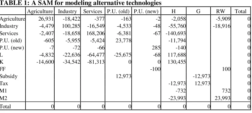
Table 1 presents the SAM. The rows show markets and the columns budgetary

constraints. Notice that the subsidy granted to the public utilities in government hands is

represented as a positive entry of $12973 in the corresponding column. H, PU, RW and

G stand for Household, Public Utility and Rest of the World and Government, and L, K

and FF for labor, specific capital and mobile capital respectively. M1 and M2 represent

imports; in this version we do not have imports of intermediate goods to be used by

industries.

TABLE 1: A SAM for modeling alternative technologies

Agriculture Industry Services P.U. (old) P.U. (new) H G RW Total Agriculture 26,931 -18,422 -377 -163 -2 -2,058 -5,909 0 Industry -4,479 100,285 -16,549 -4,533 -48 -55,760 -18,916 0 Services -2,407 -18,658 168,206 -6,381 -67 -140,693 0 P.U. (old) -605 -5,955 -5,424 23,778 -11,794 0

P.U. (new) -7 -72 -66 285 -140 0

L -4,832 -22,636 -64,477 -25,675 -68 117,688 0

K -14,600 -34,542 -81,313 0 0 130,455 0

FF -100 100 0

Subsidy 12,973 -12,973 0

Tax -12,973 12,973 0

M1 -732 732 0

M2 -23,993 23,993 0

Total 0 0 0 0 0 0 0 0 0

The state companies technology produces slightly more than 1% of total sales of

infrastructure services ($285 of $24063), and receives a subsidy from the government of

about 35% of total costs. This subsidy is financed with a tax on the household’s income.

5. Alternative technologies and model solutions.

The first solution involves computing the initial subsidy that maintains the state

owned company working at its observed levels however its inefficiency. Service

obligations are met with the installed technology, less efficient in use of intermediate

inputs and labor than the imported one.

For the initial benchmark calibration we assume that LR is used in fixed

coefficients in the domestic estate company, so that instead of (12) we have the non

negativity condition:



The subsidy s is computed initially so that the excess of costs of the state owned

enterprise are compensated and its production is equal to observed quantities. That is, s

is determined to replicate given productions of the estate owned enterprise and of the

private owned company; for example, if 70% of total production is obtained from the

state owned company, and the rest from the alternative technology, s is computed to

households income; this first simulation assumes therefore that taxes do not create costs

of distortion.

The alternative technology exhibits constant returns to scale, and uses domestic

intermediate inputs and mobile capital to produce the regulated good or service. For this

technology we also assume fixed coefficients in this presentation, and the price is fixed

at its cost of production:



where the *) stands for the input coefficients of the mobile capital technology, and p*Ris

the price of the infrastructure service when produced with the imported standards.

It is assumed that the rate of profit is given at the level of the cost of opportunity

of capital in the rest of the world, and that capital in the regulated sector is no longer

sunk. It is an implicit cost-plus mechanism with a minimum rate of return given by the

international productivity of capital. In this case KR becomes a variable to be

determined; it will be included in equation (11) in the definition of profits, with a cost

given by w*. The variable will also enter in equation (23), since it is part of the uses of

capital of the rest of the world. The trade balance equilibrium condition becomes

simply:

pT x – pm m = R + w*KR.

Given the initial subsidy s, the simulations explore the effects of assuming

reductions in w*. Changes in w*are compensated in order not to change relative prices

of exports and imports. The model chooses the less costly between the internal cost of

the subsidy and the alternative technology, to maximize welfare of the domestic

household.

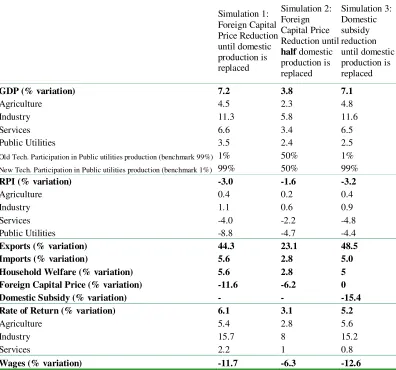
Table 2 shows the results of three simulations. The first two explore a threshold

for the cost of mobile capital: which is the level of w* such that the local public

technology is substituted by the new imported technology? The first scenario

contemplates full substitution and the second, only partial. Initially we calibrate the

model so that 99% of the total production of utilities is provided using the old

when those percentages are reverted (we do not take 100% to avoid potential

computational problems). It can be seen that a reduction of approximately 12% in the

rate of return of the rest of the world capital leads to a full replacement, and about the

half of that reduction is needed to replace half of the share. Both simulations take as

given the initial subsidy for the state owned enterprise.

However, it can be argued that the subsidies is conditional to the “international

price” of the service. In fact, though the public service cannot be imported, mobile

capital can be internalised to produce domestically. Therefore, the cost of one unit of

service produced with the new technology puts an implicit cap on the domestic price of

services. In that case, a reduction of w* could be followed by further reductions in s,

unless there is a quota or explicit ban to imports.

The subsidy s is an implicit rent of a sunk factor, and this explains why

admitting that it is endogenous could not lead to a substitution of the technology.

That is why we consider the third simulation. Instead of reducing w* we consider

reductions in the subsidy s for a given level of the cost of mobile capital. Notice that in

this case, the old and public technology is fully substituted when the subsidy is reduced

15%.

The results of reductions in the cost of mobile capital and in subsidies given to

old public companies are shown as gains both in GDP and in households´ welfare. The

latter is computed as the Equivalent Variation. When the new technology is fully

adopted, households enjoy welfare levels that are equivalent to initial income increases

of 5.6% and 5%.

It can be seen however that the new technology adoption is demanding for the

trade balance and requires additional export effort by the economy; this effort is

equivalent to w*KR since we assume that we are in a stationary state, so that initial entry

of capital +KR is compensated in the same period with an outflow –KR; when the

reimbursement of the principal encompasses several periods, the stress on the

forthcoming trade balances will be higher and the net effect will depend also on the

gains obtained with the initial inflows and the uses given to those funds.

Table 2 also alerts on potential conflicts. Nominal and real wages fell in all

scenarios; this is due to the need of rewarding mobile capital. Since labour is not mobile

It is important to remember that these simulations have been performed using

non distortionary taxation and so we should expect faster substitution when taxes on

subsets of goods are not charged, or when the tax structure is not even.

TABLE 2: Results of simulations

Simulation 1: Foreign Capital Price Reduction until domestic production is replaced Simulation 2: Foreign Capital Price Reduction until

half domestic production is replaced Simulation 3: Domestic subsidy reduction until domestic production is replaced

GDP (% variation) 7.2 3.8 7.1

Agriculture 4.5 2.3 4.8

Industry 11.3 5.8 11.6

Services 6.6 3.4 6.5

Public Utilities 3.5 2.4 2.5

Old Tech. Participation in Public utilities production (benchmark 99%) 1% 50% 1% New Tech. Participation in Public utilities production (benchmark 1%) 99% 50% 99%

RPI (% variation) -3.0 -1.6 -3.2

Agriculture 0.4 0.2 0.4

Industry 1.1 0.6 0.9

Services -4.0 -2.2 -4.8

Public Utilities -8.8 -4.7 -4.4

Exports (% variation) 44.3 23.1 48.5

Imports (% variation) 5.6 2.8 5.0

Household Welfare (% variation) 5.6 2.8 5 Foreign Capital Price (% variation) -11.6 -6.2 0 Domestic Subsidy (% variation) - - -15.4 Rate of Return (% variation) 6.1 3.1 5.2

Agriculture 5.4 2.8 5.6

Industry 15.7 8 15.2

Services 2.2 1 0.8

Wages (% variation) -11.7 -6.3 -12.6

6. Lessons from the exercises.

The simulations confirm that the choice of the technology to be used for

servicing infrastructure depends on deep parameters of efficiency and costs.

It does not say why state owned companies could be more inefficient than

distortions, the choice of the technology is not necessarily determined; it depends on the

magnitude of waste and on the costs in the allocation of resources relative to the price of

mobile capital (and implicitly on the export effort of the country).

The model shows that there are plausible scenarios where the selection is not

unique.

We have left aside additional characteristics related to the technologies that

could favour one or the other. For example, corruption and passive deficit could lead to

hyperinflation in a context of state owned enterprises, or chronic misallocation of

resources reduce investments and destroy the base of capital of government companies.

Also, we have not considered potential constraints on less developing countries exports,

that could also increase significantly the cost of raising foreign currency to honour the

payment of dividends to mobile capital.

We have not considered the possibility of using domestic capital to produce the

service of infrastructure; the idea was to consider extreme cases that could give a

confirmation of the basic intuition, and to check that that intuition was not rejected by

general equilibrium effects.

References.

Chisari O., A. Estache and C. Romero (1999), “Winners and Losers of Privatizations and Regulation of Utilities: Lesson from a General Equilibrium Model of Argentina,” The World Bank Economic Review 13:2, pp.357-378.

Chisari, O., A. Estache, G. Lambardi y C. Romero (2003), “Trade performance and regulatory regimes,” Anales de la Asociación Argentina de Economía Política, November

Dierker E., R. Guesnerie and W. Neuefeind (1985), “General Equilibrium When Some Firms Follow Special Rules,” Econometrica 53:6, pp.1369-1393

Esfahani H. and A. Ardakani (2004), “What Determines the Extent of Public Ownership?” University of Illinois and University of Manchester conference on “Regulation of Development and the Development of Regulation,” Illinois.

Quarterly Review of Economics and Finance.

Ginsburgh V. and M. Keyzer (1997), The Structure of Applied General Equilibrium Models, (Cambridge MA: The MIT Press).