Munich Personal RePEc Archive
Inference regarding multiple structural
changes in linear models estimated via
two stage least squares
Hall, Alastair R. and Han, Sanggohn and Boldea, Otilia
North Carolina State University, University of Manchester, UK,
Hyundai Research Institute, Tilburg University, Netherlands
20 June 2008
Online at
https://mpra.ub.uni-muenchen.de/9251/
Inference Regarding Multiple Structural Changes
in Linear Models Estimated via Two Stage Least Squares
1
Alastair R. Hall
University of Manchester2
Sanggohn Han
Hyundai Research Institute
and
Otilia Boldea
Tilburg University
June 20, 2008
1We are grateful to Denise Osborn and Eric Renault for valuable comments, and also for the comments of participants at the presentation of this paper at the World Congress of the Econometric Society, London, August 19-24, 2005, the Triangle Econometrics Conference, RTP, NC, December 2, 2005, CIREQ Conference on Generalized Method of Moments, Montreal, November 16-17, 2007, the ESRC Econometrics group seminar at the Institute of Fiscal Studies, London, the London-Oxbridge Time Series Workshop and at seminars at Erasmus University and the Universities of Birmingham and Warwick. We are also very grateful to Chengsi Zhang and Denise Osborn for providing us with the data used in the empirical example.
Abstract
In this paper, we extend Bai and Perron’s (1998, Econometrica, p.47-78) framework for
multi-ple break testing to linear models estimated via Two Stage Least Squares (2SLS). Within our
framework, the break points are estimated simultaneously with the regression parameters via
minimization of the residual sum of squares on the second step of the 2SLS estimation. We
establish the consistency of the resulting estimated break point fractions. We show that various
F-statistics for structural instability based on the 2SLS estimator have the same limiting
distri-bution as the analogous statistics for OLS considered by Bai and Perron (1998). This allows us
to extend Bai and Perron’s (1998) sequential procedure for selecting the number of break points
to the 2SLS setting. Our methods also allow for structural instability in the reduced form that
has been identifieda prioriusing data-based methods. As an empirical illustration, our methods
are used to assess the stability of the New Keynesian Phillips curve.
JEL classification: C12, C13
1
Introduction
Linear models are widely applied in the analysis of macroeconomic time series. In many cases,
at least some of the explanatory variables are correlated with the error and so the model is
estimated via Instrumental Variables (IV). While it is routine to assume in estimation that the
parameters of these models are constant over time, there are reasons why this assumption may
be questionable. In particular, it can be argued that policy changes and/or exogenous shifts may
cause realignments in the relationship between economic variables which are reflected in changes
in the parameters. Therefore, it is important to develop methods for both detecting parameter
instability and also for building models that incorporate this behaviour.
Considerable attention has focused on developing tests for structural instability within the
IV or more generally the Generalized Method of Moments (GMM) framework.1 The majority of
this literature has focused on the design of tests against alternatives in which there is structural
instability at a single breakpoint in the sample. Although these tests are also shown to have
non-trivial power against other alternatives, it is clearly desirable to develop procedures that
can discriminate between various forms of instability.
An important step in this direction is taken by Bai and Perron (1998).2 They develop
methods that are designed to test for discrete shifts in the parameters at potentially multiple
and unknown break points in the sample. Their analysis is in the context of linear regression
models estimated via Ordinary Least Squares (OLS). Within their framework, the break points
are estimated simultaneously with the regression parameters via minimization of the residual
sum of squares. Bai and Perron (1998) establish the consistency and the limiting distribution of
the resulting break point fractions. They also propose a sequential procedure for selecting the
number of break points in the sample based on various F-statistics for parameter constancy.
While not the only possible form for structural instability, the model with the discrete shifts
at multiple unknown break points has some appeal in macroeconometric applications because
it captures the case where relationships change due to changes in policy regime or exogenous
shifts. However, since Bai and Perron’s (1998) analysis is predicated on the assumption that
1Seeinter aliaAndrews and Fair (1988), Ghysels and Hall (1990), Andrews (1993), Sowell (1996) and Hall
and Sen (1999).
2Bai and Perron’s (1998) paper also contributes to the literature in statistics on change point estimation in
all explanatory variables are exogenous, their methods can not be applied to the types of linear
macroeconometric models mentioned above.
In this paper, we extend Bai and Perron’s (1998) framework to linear models estimated via
Two Stage Least Squares (2SLS) and thereby provide a methodology for estimating linear models
with endogenous regressors that exhibit discrete shifts in the parameters at multiple unknown
points in the sample. Within our framework, the break points are estimated simultaneously with
the regression parameters via minimization of the residual sum of squares on the second step of
the 2SLS estimation. We establish the consistency of the resulting break point fractions. We show
that the various F-statistics for testing parameter constancy based on the 2SLS estimator have
the same limiting distribution as the analogous statistics for OLS considered by Bai and Perron
(1998). This allows us to extend Bai and Perron’s (1998) sequential procedure for selecting the
number of break points to the 2SLS setting.
As can be seen from the above summary, our focus is on the stability of the parameters in
the second stage regression or, in other words, in the structural equation of interest. However
to implement 2SLS, it is necessary in the first stage regression to estimate the reduced form for
the endogenous regressors in the structural equation of interest and this, of course, requires an
assumption about the constancy or lack thereof of these reduced form parameters. In this
paper, we establish the aforementioned results under two scenarios of interest, namely: (i)
the parameters in the first stage regression are constant; (ii) the parameters in the first stage
regression are subject to discrete shifts within the sample period and the locations of these shifts
are estimated a priori via a data-based method that satisfies certain conditions. The latter
conditions allow the case in which the location of the instability is estimated via an application
of Bai and Perron’s (1998) methods to the appropriate reduced form equations on an equation
by equation basis.
To illustrate our methods, we consider the stability of the New Keynesian Phillips curve
(NKPC) estimated using quarterly data for the US over the period 1968.3-2001.4. The NKPC
is of considerable theoretical importance in monetary policy analysis and its estimation has
received considerable attention in the literature. Zhang, Osborn, and Kim (2007) observe that
empirical studies of the NKPC often reach conflicting conclusions about the importance of key
variables in the determination of inflation, and argue this may be due to neglected parameter
cause changes in the parameters of the NKPC; if true, this would mean that the parameters
of the NKPC would exhibit discrete shifts at potentially multiple points in the sample. Zhang,
Osborn, and Kim (2007) investigate this issue using a methodology based on uncovering break
points in the sample via the maximization of Wald statistics for parameter change associated
with 2SLS estimation. However, while their methodology has an intuitive appeal, there is no
theoretical justification for their methods as they note; it is, therefore, unclear exactly how to
interpret their results. In contrast, our methods can be applied to this model under plausible
assumptions about the data. Our analysis indicates that there are shifts in the parameters of
both the appropriate reduced forms and also in the NKPC itself.
It is useful to compare our results to two other recent extensions of Bai and Perron’s (1998)
framework. Qu and Perron (2007) extend Bai and Perron’s (1998) framework to systems of
regression equations and consider the case in which estimation and inference are based on
quasi-maximum likelihood techniques under normality. Perron and Qu (2006) consider the case of a
regression equation in which the least squares estimation imposes cross-regime restrictions, such
as the equality of parameters in two non-adjacent regimes. While both these papers expand
the set of available techniques in important ways, both sets of results are predicated on the
assumption that the explanatory variables are uncorrelated with the error(s). To our knowledge,
our paper is the first to consider estimation and inference about multiple structural changes in
a linear model with endogenous regressors.
An outline of the paper is as follows. Section 2 lays out the model, illustrates it via the NKPC
and also explains details of the estimation. Section 3 presents results on the limiting behaviour
of the break fraction estimators associated with the 2SLS estimation of the structural equation
of interest. It is shown that the break fraction estimators are consistent and deviate from the
true break fractions by a term of large order in probability T−1, where T is the sample size.
The import of this result is that inference regarding the parameters of the structural equation
can be conducted as if the the true break fractions are known a priori. In the remainder of
the paper, we consider the limiting behaviour of the 2SLS estimator and various associated
inference procedures. Section 4 presents the limiting distribution of the 2SLS estimator. Section
5 presents the limiting distributions of the various F-statistics. The simulation evidence is
reported in Section 6. Section 7 presents our empirical application and some concluding remarks
2
The Model and The Estimation
2.1
The model
We consider the case in which the equation of interest is a multiple linear regression model with
m breaks (i.e. m+ 1 regimes), that is
yt = x′tβx,i0 + z′1,tβ0z1,i +ut, i= 1, ..., m+ 1, t=T
0
i−1+ 1, ..., Ti0 (1)
where T0
0 = 0 and Tm0+1 = T. In this model, yt is the dependent variable, xt is a p1×1
vector of explanatory variables that are correlated with the error ut andz1,t is ap2×1 vector
of explanatory variables that are uncorrelated with ut and includes the intercept. We define
p=p1+p2. The error term, ut, is assumed to have a mean of zero.
Following the convention in the literature, we index the break points{T0
i}by break fractions
{λ0
i}. These break fractions must satisfy the following:3
Assumption 1 T0
i = [T λ0i], where0< λ01< ... < λ0m<1.
Assumption 1 requires the break points to be asymptotically distinct.
In view of the correlation betweenxt andut, OLS estimation of (1) would yield inconsistent
estimators of the regression parameters. We therefore consider the case in which (1) is estimated
via 2SLS. To implement 2SLS, it is necessary to specifiy the reduced form for x. As noted in
the introduction, we consider two scenarios: (i) the reduced form for xt is structurally stable;
(ii) the reduced form forxtexhibits parameter variation. We elaborate on these two scenarios
in turn.
Scenario (i): stable reduced form.
The reduced form forxtis assumed to be as follows:
x′
t = z′t∆0 +vt′ (2)
where zt = (zt,1, zt,2, ..., zt,q)′ is a q×1 vector of instruments that is uncorrelated with both
ut and vt, ∆0 = (δ1,0, δ2,0, ..., δp1,0) with dimension q×p1 and each δj,0 for j = 1, ..., p1 has
dimension q×1. We assume thatzt containsz1,t. Under the assumption thatE[ut2|zt] =σ2,
the optimal IV estimator is the 2SLS estimator.4 Our analysis is confined to the 2SLS estimator,
although we wish to emphasize that the aforementioned conditional homoscedasticity restriction
is only imposed in certain parts of the analysis. ⋄.
Scenario (ii): unstable reduced form.
The reduced form forxtis:
x′t = z ′ t∆
(i) 0 +v
′
t, i= 1,2, . . ., h+ 1, t=Ti∗−1+ 1, . . ., Ti∗ (3)
where T∗
0 = 0 and Th∗+1=T. The points{Ti∗}are assumed to be generated as follows.
Assumption 2 T∗
i = [T π0i], where0< π10< . . . < π0h<1.
Note that the break fractions{π0
i}may or may not coincide with{λ0i}. Letπ0= [π01, π02, . . . , π0h]′.
Within our analysis, it is assumed that the break points in the reduced form are estimated prior
to estimation of the structural equation in (1). For our analysis to go through, the estimated
break fractions in the reduced form must satisfy certain conditions that are detailed below; these
conditions would hold, for instance, if Bai and Perron’s (1998) methodology is applied equation
by equation to the reduced form.
Equation (3) can be re-written as follows
x′t = ˜zt(π0) ′
Θ0 + v
′
t, t= 1,2, . . ., T (4)
where Θ0 = [∆(1)
′
0 ,∆ (2)′
0 , . . . ,∆ (h+1)′
0 ]
′
, ˜zt(π0) =ι(t, T)⊗zt,ι(t, T) is a (h+ 1)×1 vector with
first elementI{t/T ∈(0, π0
1]},h+1thelementI{t/T ∈(π0h,1]},kthelementI{t/T ∈(πk0−1, πk0]}
for k= 1,2, . . ., handI{·}is an indicator variable that takes the value one if the event in the curly brackets occurs. Notice that (4) fits the generic constant parameter form of (2). ⋄
To illustrate the potential interest in our framework, we consider the case of the NKPC. For ease
of exposition, it suffices here to consider the following stylized version of the NKPC,
inft = c0 + αfinfte+1|t +αbinft−1 +αogogt +ut (5)
where inft is inflation in (time) period t, infte+1|t denotes expected inflation in period t+ 1
given information available in period t, ogt is the output gap in period t, utis an unobserved
error term andθ= (c0, αf, αb, αy)′are unknown parameters. The variablesinfte+1|tandogtare
see Zhang, Osborn, and Kim (2007) and the references therein. Suitable instruments must be
both uncorrelated withutand correlated withinfte+1|t andogt. In this context, the instrument
vector zt commonly includes such variables as lagged values of expected inflation, the output
gap, the short-term interest rate, unemployment, money growth rate and inflation. This model
fits within our framework with (5) as the structural equation of interest provided the reduced
forms forinfe
t+1|tandogtare assumed to be given by either (2) or (3). We return to this example
in Section 7.
2.2
The estimation
To describe the estimation of the model, it is assumed that the number of break points m is
known but their location is not. Therefore the researcher must estimate both the break points
and regression parameters. This estimation proceeds as follows. On the first stage, the reduced
form for xt is estimated via OLS using - as appropriate - either (2) or a version of (4) with
estimated break fractions substituted for π0. Let ˆx
t denote the resulting predicted value for
xt. The second stage of the 2SLS estimation is itself divided into a number of steps because of
the need to estimate both the break points and the regression parameters. The first step of the
second stage is to estimate the model
yt = ˆx ′
tβx,i∗ +z1′,tβ∗z1,i + ˜ut, i= 1, ..., m+ 1; t=Ti−1+ 1, ..., Ti (6)
via OLS for each possiblem-partition of the sample, denoted by{Tj}mj=1, such thatTi−Ti−1≥q.
Lettingβi∗
′
= (βx,i∗
′ , βz∗1,i
′
)′, the resulting estimates ofβ∗= (β1∗
′ , β2∗
′
, ..., β∗m+1
′
)′are obtained by
minimizing the sum of squares of the residuals
ST(T1, ..., Tm) = m+1
X
i=1
Ti
X
t=Ti−1+1
(yt−xˆ′tβx,i−z′1,tβz1,i)
2 (7)
with respect toβ= (β1′, β2′, ..., βm+1′)
′
. We denote these estimators by ˆβ({Ti}mi=1).
The second step of the second stage involves constructing the minimized sum of squares
associated with (6) for each partition, that is
ST(T1, ..., Tm; ˆβ({Ti}mi=1) =
m+1
X
i=1
Ti
X
t=Ti−1+1
(yt−xˆ′tβi−z′1,tβz1,i)
2 β= ˆβ({T
i}mi=1)
The estimates of the break points, ( ˆT1, ...,Tˆm), are defined as
( ˆT1, ...,Tˆm) = arg min T1,...,Tm
ST(T1, ..., Tm; ˆβ({Ti}mi=1)) (9)
where the minimization is taken over all partitions, (T1, ..., Tm) such that Ti−Ti−1 ≥q. The
2SLS estimates of the regression parameters, ˆβ({Tˆi}mi=1) = ( ˆβ1′,βˆ2′, ...,βˆ′m+1)′, are the regression
parameter estimates associated with the estimated partition,{Tˆi}mi=1.
3
Limiting behaviour of the break fraction estimators
In this section we analyze the limiting behaviour of the break point fraction estimators {λˆi =
ˆ
Ti/T}. Two properties are established: consistency and that the estimated break fractions
de-viate from the true break fractions by an Op(T−1) term. These results are established for both
the scenarios regarding the parameters of the reduced form for xt described in Section 2. We
take each of these scenarios in turn.
3.1
Stable reduced form
In this case, the predicted value forxt is given by
ˆ
x′t = zt′∆ˆT = zt′( T
X
t=1
ztzt′)−1 T
X
t=1
ztxt′ (10)
To facilitate the analysis of this version of the model, we impose the following conditions.
Assumption 3 Letbt= (ut, vt′)′ and F =σ−field{. . . , zt−1, zt, . . . , bt−2, bt−1}. Assume btis
a martingale difference relative to {Ft}and suptE[kbtk4]<∞.
Assumption 4 rank{[∆0,Π]}=pwhereΠ′= [Ip2,0p2×(q−p2)],Ia denotes thea×aidentity
matrix and0a×b is the a×b null matrix.
Assumption 5 There exists an l0 > 0 such that for all l > l0, the minimum eigenvalues of
Ail = (1/l)PT
0
i+l
t=T0
i+1ztzt
′ and of A∗
il = (1/l)
PTi0
t=T0
i−lztzt
′ are bounded away from zero for all
i= 1, ..., m+ 1.
Assumption 6 T−1P[T r]
t=1ztz
′
t p
→ QZZ(r) uniformly in r ∈ [0,1] where QZZ(r) is positive
Assumption 7 The minimization in (9) is over all partitions(T1, ..., Tm)such thatTi−Ti−1>
ǫT for someǫ >0and ǫ < infi(λ0i+1−λ0i).
A few comments on these assumptions are in order. Assumption 3 includes the restrictions
thatbtis a serially uncorrelated process, and hence the errors in both the structural equation and
reduced form exhbit this property. This assumption also includes the restriction that E[ztb′t] =
0q×(p1+1) which implies both the implicit population moment condition in 2SLS is valid - that
is E[ztut] = 0 - and also that the conditional mean of the reduced form is correctly specified.
However, note that this assumption does allowzt to contain lagged values ofyt. Assumption 4
implies the standard rank condition for identification in IV estimation in the linear regression
model5because Assumptions 3, 4 and 6 together imply that
T−1
[T r]
X
t=1
zt[x′t, z1′,t] ⇒ QZZ(r)[∆0,Π] = QZ,[X,Z1](r) uniformly inr∈[0,1]
where QZ,[X,Z1](r) has rank equal to p for any r > 0. Assumption 5 requires that there be
enough observations near the true break points so that they can be identified. This condition
is analagous to Bai and Perron’s (1998) Assumption A2 and the interested reader is refered to
this source for further discussion of this condition. Assumption 7 requires that each segment
considered in the minimization contains a positive fraction of the sample asymptotically; in
practice ǫis chosen to be small in the hope that the last part of the assumption is valid.
The proof strategy for consistency is identical to that used by Bai and Perron (1998) in their
proof of the corresponding results for OLS estimators. The proof builds from the following two
properties of the error sum of squares on the second stage of the 2SLS esimation.
• Since the 2SLS estimators minimize the error sum of squares in (7), it follows that
(1/T)
T
X
t=1
ˆ
u2
t ≤ (1/T) T
X
t=1
˜
u2
t (11)
where ˆut=yt−ˆx ′
tβˆx,j−z1′,tβˆz1,jdenotes the estimated residuals fort∈[ ˆTj−1+1,Tˆj] in the
second stage regression of 2SLS estimation procedure and ˜ut=yt−xˆ ′
tβx,i0 −z′1,tβz01,idenotes
the corresponding residuals evaluated at the true parameter value fort∈[T0
i−1+ 1, Ti0].
• Usingdt= ˜ut−uˆt= ˆx ′
t( ˆβx,j−βx,i0 )−z ′
1,t( ˆβz1,j−β
0
z1,i) overt∈[ ˆTj−1+1,Tˆj]∩[T
0
i−1+1, Ti0],
it follows that
T−1
T
X
t=1
ˆ
u2t = T−1 T
X
t=1
˜
u2t +T−1 T
X
t=1
dt2 − 2T−1 T
X
t=1
˜
utdt (12)
Consistency is established by proving that if at least one of the estimated break fractions does
not converge in probability to a true break fraction then the results in (11)-(12) contradict each
other. This conflict is established using the results in the following lemma.
Lemma 1 Let yt be generated by (1), xt be generated by (2), xˆt be generated by (10) and
Assumptions 1, 3-7 hold.
(i) T−1PT
t=1u˜tdt=op(1).
(ii) If ˆλj 6 p
→λ0
j for somej, then
lim sup
T→∞
P T−1
T
X
t=1
dt2> Ck∆0(βx,j0 −β0x,j+1)k2 + kβ0z1,j −β
0
z1,j+1k
2 +ξ
T
!
>¯ǫ
for someC >0and ¯ǫ >0, whereξT =op(1).
Using (11)-(12) and Lemma 1, consistency is established along the lines anticipated above.
Theorem 1 Let yt be generated by (1), xt be generated by (2), xˆt be generated by (10) and
Assumptions 1, 3-7 hold, then λˆj
p
→λ0
j for all j= 1,2, ..., m.
For the development of inference procedures for determining the number of breaks, it is important
to know not only that the break fraction estimators are consistent but also the order of magnitude
of their deviation from the true break fraction. This is established in the following theorem.
Theorem 2 Let yt be generated by (1), xt be generated by (2), xˆt be generated by (10) and
Assumptions 1, 3-7 hold then, for everyη >0, there existsC such that for all largeT,P(T|ˆλj−
λ0
j|> C)< η, forj= 1, ..., m.
Therefore, the break fraction estimators deviate from the true break fractions by a term of order
3.2
Unstable reduced form
Recall that the reduced form exhibits discrete parameter changes at unknown points in the
sample and these points are indexed by the break fraction vector, π0. We suppose that π0 is
estimated by ˆπand that these estimated break fractions satisfy the following condition.
Assumption 8 πˆ = π0 +O
p(T−1)
Note that Assumption 8 implies ˆπis consistent forπ0 andT(ˆπ−π0) is bounded in probability.
Such an estimator might be obtained by applying Bai and Perron (1998)’s methodology equation
by equation and then pooling the resulting estimates of the break fractions. For our purposes,
it only matters that Assumption 8 holds and not how ˆπis obtained. The latter is, of course, a
matter of practical importance but we do not address it here.
These estimated breaks are imposed on the the reduced form forxt. Let ˆΘT be the OLS
estimator of Θ0 from the model
x′t = ˜zt(ˆπ)′Θ0+error t= 1,2,· · ·, T (13)
where ˜zt(ˆπ) is defined analogously to ˜zt(π0), and now define ˆxtto be
ˆ
x′
t = ˜zt(ˆπ)′ΘˆT = ˜zt(ˆπ)′{ T
X
t=1
˜
zt(ˆπ)˜zt(ˆπ)′}−1 T
X
t=1
˜
zt(ˆπ)x′t (14)
For the analysis in the case, the regularity conditions need to be altered. Assumption 4 is
replaced by:
Assumption 9 rankn h∆(0i),Π
i o
=pfori= 1,2,· · ·, h+ 1and Πis defined in Assumption 4.
It is also necessary to modify Assumption 7.
Assumption 10 The minimization in (9) is over all partitions(T1, ..., Tm)such thatTi−Ti−1>
ǫT for someǫ >0and ǫ < infi(λ0i+1−λi0)and ǫ < infj(π0j+1−π0j).
The following theorem establishes the consistency of the break fraction estimators.
Theorem 3 If Assumptions 1-3, 5-10 hold,ytis generated via (1), xtis generated via (4) and
ˆ
xt is calculated via (14), then
ˆ
λj p
→λ0
In order to extend Theorem 2, we impose one final condition.
Assumption 11 There exists an l∗ >0 such that for all l > l∗, the minimum eigenvalues of
Bil = (1/l)PT ∗
i+l
t=T∗
i+1ztzt
′ and of B∗
il = (1/l)
PTi∗
t=T∗
i−lztzt
′ are bounded away from zero for all
i= 1, ..., h+ 1.
Assumption 11 is similar to Asssumption 5 above but refers to the break points in the reduced
form. The order in probability of the estimated break fractions is given in the following theorem.
Theorem 4 If Assumptions 1-3, 5-11 hold, yt is generated via (1), xt is generated via (4)
and xˆt is calculated via (14), then, for every η > 0, there exists C such that for all large T,
P(T|λˆj−λ0j|> C)< η, for j= 1, ..., m.
3.3
Discussion
At this stage, it is useful to comment on the nature of the foregoing analysis. First consider the
case where the reduced form is structurally stable. In this case, Theorems 1-2 establish that
the break fraction estimators, {λˆj}, are consistent and ˆλj−λ0j =Op(T−1). Now consider the
case where the reduced form exhibits parameter variation. If the location of the breaks in the
reduced form are knowna priorithen, as noted above, the reduced form can be re-written as a
structurally stable regression equation involving the augmented parameter vector.6 Therefore, in
this case, the limiting behaviour of the break fraction estimators associated with the structural
equation is covered by Theorems 1-2. However, in most cases, the locations of the breaks in
the reduced form are unknown and so must be estimated a priori. In this case, Theorems 3-4
provide conditions on the estimators of the reduced form break fractions, {πˆi}, under which
the break fraction estimators associated with the structural equation, {λˆj}, are consistent and
ˆ
λj−λ0j =Op(T−1).
Of the scenarios described above, the most empirically relevant is likely to be the one
in-volving estimation of break fractions in both reduced form and structural equations. Under our
assumptions, the estimators of the break fractions in both reduced form and structural equations
converge at rate T to the true break fractions. It emerges below that this rate is sufficiently
fast that the estimation of the break fractions can be ignored in the asymptotic analysis of the
2SLS estimators and its associated statistics.7 In other words, for the purposes of the
asymp-totic analysis of the 2SLS estimator and its associated statistics, we can essentially proceed as
if the break fractions in both equations are known. Since, as noted above, the reduced form
with known break points can be rewritten as a constant parameter regression model, we focus
exclusively for the remainder of the paper on the case in which the reduced form is structurally
stable. The analagous results for the model with parameter variation in the reduced form can
be deduced from the results presented with an appropriate redefinition of the regressor vector in
the reduced form.
4
The limiting distribution of the 2SLS estimators
Once the break fractions are estimated, it is clearly desirable to perform inference about the
structural parameters {β0
i}. If the break fractions are known a priorithen standard arguments
can be employed to show the root T asymptotic normality of the 2SLS estimator. Since the
estimated break fractions converge at rate T, this standard asymptotic distribution theory can
be extended to the 2SLS estimates based on the estimated break fractions.
Theorem 5 Let yt be generated by (1), xt be generated by (2), xˆt be generated by (10) and
Assumptions 3-6 hold, then
T1/2βˆ({Tˆi}mi=1) − β0
=⇒ N 0p(m+1)×1, Vβ
where β0= [β0 1
′ , β0
2
′ , . . . , β0
h+1
′
]′,β0
i = [βx,i0
′ , β0
z1,i
′
]′,
Vβ =
Vβ(1,1) · · · Vβ(1,m+1) ..
. . .. ...
Vβ(m+1,1) · · · Vβ(m+1,m+1)
Vβ(i,j) = RiS(i,j)R′j, fori, j= 1,2, . . .m+ 1
Ri = A(1)QZZ(1)−1QiQZZ(1)−1A(1)′
−1
A(1)QZZ(1)−1
and Qi=QZZ(λ0i)−QZZ(λ0i−1),A(r)′= [QZX(r), QZ1Z(r)
′],Q
Z1Z(r)is the probability limit of
T−1P[T r]
t=1z1,tz′t(defined in Assumption 6),S(i,j)=limT→∞Cov[T−1/2Pi0ztu˜t, T
−1/2P
j0ztu˜t],
P
i0 denotes the summation overt= [T λ
0
i−1] + 1, . . .[T λ0i], and we setλ00 = 0,λ0m+1= 1.
Note thatS(i,j)is non-zero in general because the first stage regression pools observations across
regimes and this creates a connection between the aforementioned sums from different regimes.
However, if the reduced form is also unstable then the connection across regimes is broken in
one leading case. If the breaks in the structural equation also occur in the reduced form then
the predictions are only based on the observations in the sub-sample in question and so Vβ is
block diagonal. Specifically, ifh≥mandλ0
i =π0j for somej for each ithen
Vβ = diag( ˜Vβ(1,1),V˜
(2,2)
β , . . . ,V˜
(m+1,m+1)
β ) (15)
where ˜Vβ(i,i) = ˜RiS˜(i,i)R˜′i, ˜Ri = AiQ−i1A′i
−1
AiQ−i 1, Ai = A(λ0i)−A(λ0i−1), and ˜S(i,i) =
limT→∞T−1Pi0V ar[ztut]. Notice that ˜V
(i,i)
β is just the variance of the 2SLS estimator based
on theithsub-sample allowing potentially for breaks in the reduced form within that sub-sample.
5
Test statistics for multiple breaks
The sup-F type test of no structural break (m= 0) versus the alternative hypothesis that there
is m = 1 break has been considered by Andrews (1993). Bai and Perron (1998) generalize
Andrew’s sup-F type test to the hypothesism=kfor linear models estimated via OLS. In this
section, we extend Bai and Perron’s results to linear models estimated via 2SLS.
For this part of the analysis, we impose the following restrictions.
Assumption 12 (i) T−1P[T r]
t=1ztz′t p
→rQZZ uniformly in r∈[0,1]whereQZZ is a positive
definite matrix of constants;
(ii) the conditional variance of the errors is independent oft, that is
V ar
ut
vt
zt
= Ω =
σ2 γ′
γ Σ
whereΩis a constant, positive definite matrix,σ2 is a scalar and Σis ap
1×p1 matrix;
The restrictions in Assumption 12 are analogous to that imposed by Bai and Perron (1998) in
their Assumptions A8 and A9 which underpin their analysis of various F-statistics for testing
for multiple breaks within the OLS framework.8
8Although note that the conditional variance restriction in Assumption 12 involves bothu
t andvt whereas
Assumptions 3 and 12 together ensure that a uniform version of the multivariate functional
central limit theorem in de Jong and Davidson (2000) holds:
T−1/2
[T r]
X
t=1
ut
vt
⊗zt =⇒ (Ω
1/2⊗Q1/2
ZZ)Bn(r) (16)
whereBn(r) is an×1 standard Brownian motion withn=q×(p1+ 1) and “=⇒” denotes weak
convergence in the spaceD[0,1] under the skorohod metric.
The sup-F type test statistic can be defined as follows. Let (T1, ..., Tk) be a partition such
that Ti = [T λi] (i= 1, ..., k). Define
FT(λ1, ..., λk;p) =
T−(k+ 1)p
kp
SSR0−SSRk
SSRk
(17)
where SSR0 and SSRk are the sum of squared residuals based on the fitted X under null and
alternative hypothesis, respectively. Recall from Assumption 7 that the minimization is
per-formed over partitions which are asymptotically large and the size of the partitions is controlled
by ǫ, a non-negative constant. Accordingly, we define Λǫ ={(λ1, ..., λk) :|λi+1−λi| ≥ǫ, λ1≥
ǫ, λk≤1−ǫ}. Finally, the sup-F type test statistic is defined as
Sup−FT(k;p) = Sup(λ1,...,λk)∈ΛǫFT(λ1, .., λk;p) (18)
Theorem 6 If the data are generated by (1)-(2) withm= 0,xˆt is generated by (10) and
As-sumptions 1, 3-7 and 12 hold then Sup−FT(k;p)⇒Sup−Fk,p≡Sup(λ1,...,λk)∈ΛǫF(λ1, .., λk;p)
where
F(λ1, ..., λk;p) ≡
1
kp
k
X
i=1
||λi+1Wi−λiWi+1||2
λiλi+1(λi+1−λi)
where kis the number of break points under the alternative hypothesis, andWi ≡Bp(λi).
We note that the limiting distribution in Theorem 6 is exactly the same as the one in Bai and
Perron’s (1998) analogous result for the sup-F test based on OLS estimators when the regressors
are exogenous. Percentiles for this distribution can be found in Bai and Perron (1998)[Table I]
forǫ= 0.05 and in Bai and Perron (2001) for other values ofǫ.
TheSup−FT(k;p) statistic is used to test the null hypothesis of structural stability against
thek-break model, and so is designed for the case in which a particular choice ofkis of interest.
for the alternative hypothesis. To circumvent this problem, Bai and Perron (1998) propose so
called “Double Maximum tests” that combine information from theSup−FT(k;p) statistics for
different values of k running from one to some ceilingK. We consider here only the following
example of Double Maximum test,9
U DmaxFT(K;p) = max
1≤k≤K(λ sup
1,...,λk)∈Λǫ
FT(λ1, ..., λk;p) (19)
The limiting distribution of this statistic follows directly from Theorem 6.
Corollary 1 Under the conditions of Theorem 6, it follows that
U DmaxFT(K;p) =⇒ max
1≤k≤K{Sup−Fk,p}
Critical values for the limiting distribution in Corollary 1 are presented in Bai and Perron
(1998)[Table 1] for ǫ= 0.05 and in Bai and Perron (2001) for other values ofǫ.
TheSup−FT(k;p) and U DmaxFT(K;p) statistics are used to test the null hypothesis of
no breaks. It is also of interest to develop statistics for testing the null hypothesis of l breaks
against the alternative ofl+ 1 breaks. Following Bai and Perron (1998), a suitable statistic can
be constructed as follows. For the model withl breaks, the estimated break points, denoted by
ˆ
T1, ...,Tˆl, are obtained by a global minimization of the sum of the squared residuals as in (9).
For the model withl+ 1 breaks,lof the breaks are fixed at ˆT1, ...,Tˆland then the location of the
(l+ 1)th break is chosen by minimizing the residual sum of squares. The test statistic is given
by
FT(l+ 1|l) = max
1≤i≤l+1{
SSRl( ˆT1, ...,Tˆl)−infτ∈Λi,ηSSRl+1( ˆT1, ...,Tˆi−1, τ,Tˆi, ...,Tˆl)} ˆ
σ2
i
} (20)
where
ˆ
σ2
i =
ˆ
Ti
X
t= ˆTi−1+1
(yt−xˆ ′
tβˆx,i−z1′,tβˆz1,i)
2/( ˆT
i−Tˆi−1−p)
Λi,η = {τ : ˆTi−1+ ( ˆTi−Tˆi−1)η≤τ ≤Tˆi−( ˆTi−Tˆi−1)η}
and ˆβi is the 2SLS estimator calculated using the sample ˆTi−1+ 1, . . . ,Tˆi on the second stage.
The following theorem gives the limiting distribution of this statistic under the null hypothesis
of lbreaks.
9UDmax denotes Unweighted Double maximum. Bai and Perron (1998) also consider a WDmax statistic
in which the the maximum is taken over weighted values of theSup−FT(k;p) statistics. AnalogousWDmax
Theorem 7 If the data are generated by (1)-(2) with m =l,xˆt is generated by (10) and
As-sumptions 1, 3-7 and 12 hold then then limT→∞P(FT(l+ 1|l)≤x) =Gp,η(x)l+1 whereGp,η(x)
is the distribution function of supη≤µ≤1−ηkW(µ)−µW(1)k2/µ(1−µ)and W(µ)≡Bp(µ).
Once again, the limiting behaviour of the test statistic is the same as that of the analogous
statistic proposed by Bai and Perron (1998) for the OLS case. Critical values can be found in
Bai and Perron (1998)[Table II] for the case in which calculated with η =.05 and in Bai and
Perron (2001) for other values ofη.
Following Bai and Perron (1998), the statistics described in this section can be used to
determine the estimated number of breakpoints, ˆkT say, via the following sequential strategy.
On the first step, use eitherSup−FT(1;p) orU DmaxFT(K, p) to test the null hypothesis that
there are no breaks. If this null is not rejected then ˆkT = 0; else proceed to the next step. On
the second step FT(2|1) is used to test the null hypothesis that there is only one break against
the alternative hypothesis of two breaks. If FT(2|1) is insignificant then ˆkT = 1; else proceed
to the next step. On the lth step F
T(l+ 1|l) is used to test the null hypothesis that there are
l breaks against the alternative hypothesis of l+ 1 breaks. If FT(l+ 1|l) is insignificant then
ˆ
kT =l; else proceed to the next step. This sequence is continued until some preset ceiling for
the number of breaks,Lsay, is reached. If all statistics in the sequence are significant then the
conclusion is that there are at leastLbreaks. We evaluate the finite sample performance of this
strategy as part of the simulation study reported in the following section.
To conclude our discussion of these F-statistics, we return to the issue of the assumptions on
the errors. Assumption 12 requires the errors to be homoscedastic and serially uncorrelated. It
is, however, possible to relax this assumption to some extent as we now discuss. Suppose that it
is assumed that a regime is characterized by both a change in the regression parameter vector
and also a change in the conditional variance matrix of the errors, that is Ω in Assumption
12 is replaced by Ωi for t ∈ [T λ0i−1] + 1,[T λ0i]
. Since the calculation of FT(l+ 1|l) only
involves sub-sample covariance matrix estimators, it follows that the limiting distribution of the
test statistic is unaffected by heteroscedasticity of this type. It is therefore possible to use the
the test statistics described above to develop a sequential strategy to determine the number of
breaks for the case where the no break model is homoscedastic and thel break models involve
6
Finite sample behaviour
In this section, we evaluate the finite sample behaviour of the various statistics discussed in
the previous sections via a small simulation study. The simulation design involves models with
zero, one or two breaks. Since our analysis of the break fractions is premised on the existence
of a break, we begin by discussing the one break and two break models. We then conclude the
sections by considering the behaviour of the test statistics in the no break model.
6.1
One break model
The data generating process for the structural equation is:
yt = [1, xt]′β10 +ut, fort = 1, . . . ,[T /2]
= [1, xt]′β20 +ut, fort = [T /2] + 1, . . . , T
(21)
The reduced form equation for the scalar variablextis:
xt = zt′δ + vt, fort= 1, . . ., T (22)
whereδ isq×1. The errors are generated as follows: (ut, vt) ′
∼IN(02×1,Ω) where the diagonal
elements of Ω are equal to one and the off-diagonal elements are equal to 0.5. The instrumental
variables, zt, are generated via: zt ∼ i.i.d N(0q×1, Iq). The specific parameter values are as
follows: (i) T = 60,120,240,480; (ii) (β0
1, β20) = ([1,0.1]′,[−1,−0.1]′); (iii)q = 2,4,8; (iv)δ is
chosen to yield the population R2 = 0.5 for the regression in (22).10 For each configuration,
1000 simulations are performed.
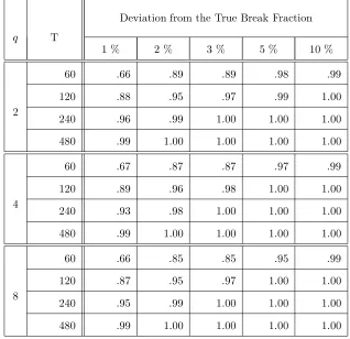
The results are presented in Tables 1-4. We first consider the behaviour of the break fraction
estimator calculated under the assumption that there is only one break. Table 1 reports the
proportion of the simulations in which |λˆ1−λ01| ≤c forc= 0.01,0.02,0.03,0.05,0.1. It can be
seen that in the smallest sample size (T = 60) there is some dispersion but the proportions clearly
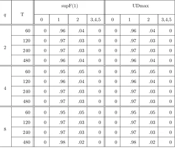
increase withT and exhibit behaviour in line with the consistency result in Theorem 1. Table 2
reports the relative rejection frequencies ofSup−FT(k; 1) (for k= 1,2),U DmaxFT(5; 1) and
FT(l+ 1|l) (forl= 1,2) statistics where, in both cases the nominal size is 0.05. Notice that the
10For this model,δ=p
alternative hypothesis is true for theSup−FT(k; 1) andU DmaxFT(5; 1) statistics and so these
relative frequencies are empirical powers for this statistic. Whereas, forl= 1, the null hypothesis
is correct forFT(l+ 1|l) and so the relative frequencies are the empirical size, and forl= 2, the
null assumes more breaks than there actually are. Both Sup−FT(k; 1) and U DmaxFT(5; 1)
reject 100% of the time. The FT(2|1) statistic is close to its nominal size; FT(3|2) tends to
reject less frequently than the nominal size. Table 3 reports the results from using the sequential
strategy based on these statistics that is described in Section 5 with a maximum number of breaks
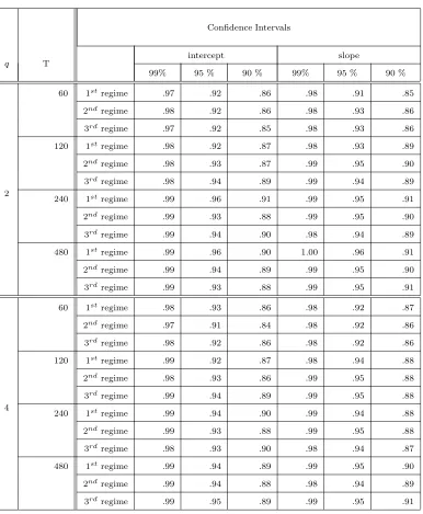
set equal to five. The results indicate that the strategy works well in each case. Table 4 reports
the empirical coverage of the large sample confidence intervals based on the limiting distribution
in Theorem 5, with all limiting covariances replaced by their empirical counterparts.11 As can
be seen, the empirical coverage is very close to the nominal level in all cases, and is within 3
simulation standard deviations of the nominal level for all confidence levels in all but the smallest
sample size.
6.2
Two break model
The data generation process for the structural equation is:
yt = [1, xt]′β10 +ut, fort = 1, . . .,[T /3]
= [1, xt]′β20 +ut, fort = [T /3] + 1, . . .,[2T /3]
= [1, xt]′β30 +ut, fort = [2T /3] + 1, . . ., T
Two choices for β0 are considered: (β0
1, β02, β30) = ( [1,0.1]′,[−1,−0.1]′,[1,0.1]′). All other
aspects of the design are the same as the one break model.
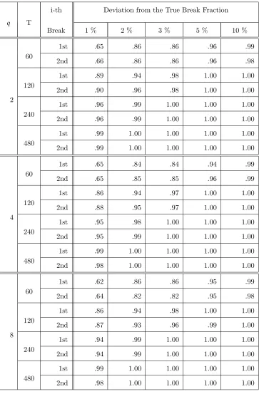
The results are reported in Tables 5-9. Again, we begin by considering the performance of
the estimated break fractions. Table 5 reveals that, as in the one break model, there is some
dispersion in the estimates of the break fractions in the smallest sample size but nevertheless the
empirical distribution of the break fraction estimator is evidently collapsing on the true fraction
11Within this model, it can be shown thatS
i,i= (λ0i−λ0i−1)
n
V1,1+ (1 +λ0i−1−λ0i) [(β0
′
i ⊗Iq)V2,2(β0i⊗Iq) + 2V1,2(βi0⊗Iq) ]
o
and S(i,j) = −(λi0−λ0i−1)(λ0j−λ0j−1)[V1,2(βj0⊗Iq) + (β0
′
i ⊗Iq)V2,1+ (β0
′
i ⊗Iq)× V2,2(βj0⊗Iq)] where
V =
V1,1 V1,2
V′ 1,2 V2,2
is the long-run covariance ofT
−1/2PT
t=1(ut, v′t)′⊗zt,V1,1isq×qandV2,2 isqp1×qp1.
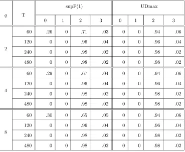
asT increases. Table 6 reports the relative rejection frequencies ofSup−FT(k; 1) (fork= 1,2),
U DmaxFT(5; 1) and FT(l+ 1|l) (for l = 1,2) statistics where, in both cases the nominal size
is 0.05. As in the one break model, the statistics are applied with k, l = 1,2. Notice that the
alternative hypothesis is true for theSup−FT(k; 1),U DmaxFT(5; 1) andFT(2|1) statistics and
so these relative frequencies are empirical powers for this statistic. Whereas, the null hypothesis
is correct for FT(3|2) and so the relative frequencies are the empirical size. From Table 6 it
can be seen that, unlike the one break model, there is a difference in the power properties of
the tests. While Sup−FT(k; 2) andU DmaxFT(5; 1) reject 100% of the time, Sup−FT(k; 1)
only rejects 74% power in the smallest sample size although it does reject 100% of the time
in larger sample sizes. The test of one break against two (FT(2|1)) also rejects 100% in every
case. The test of two breaks against three (FT(3|2)) is slightly undersized; this contrasts with
the results for FT(2|1) in the one break model and likely reflects the smaller sub-sample sizes
in the two break model. Table 7 reports the results using the sequential strategy for estimating
the number of breaks. As would be expected given the power results, the sequential strategy
starting with Sup−FT(k; 1) has a marked tendency to under estimate the number of breaks
in the smallest sample size. In contrast, the sequential strategy starting with U DmaxFT(5; 1)
works well at all sample sizes as it never underfits and picks the true order never less than 94% of
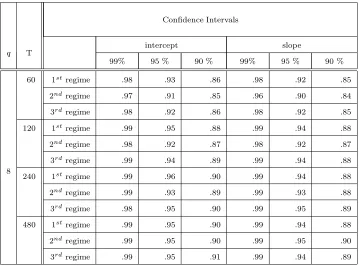
the time. Tables 8-9 report the empirical coverage of the large sample confidence intervals based
on the limiting distribution in Theorem 5. In the smallest sample size (T = 60), the coverage
is lower than the nominal level and more than three simulation standard errors away from the
nominal level; this can be explained by small sizes of the sub-samples in this case. However,
the empirical coverage is within three simulation standard errors for all intervals at the other
samples (T = 120,240,480) and very close to the nominal level in the larger samples.
6.3
No break model
The previous two designs involve cases where there is a change in the regression parameters of
the structural equation. It is also of interest to explore how the test statistics perform in the
case where there is no break and so the model is structurally constant. To this end, data are
generated from (21) with β0
1 = β20 = [1,1]. All other aspects of the design are the same as
(k= 1,2),FT(l+ 1|l) (l= 1,2) andU DmaxFT(5; 1) statistics. Note that within this design, the
null hypothesis is correct for theSup−FT(1; 1),Sup−FT(2; 1), andU DmaxFT(5,1) statistics,
and so the rejection frequency equals the empirical size. ForFT(2|1) andFT(3|2) statistics, the
null hypothesis involves more breaks than are present in the data. From Table 11, it can be
seen thatSup−FT(1; 1),Sup−FT(2; 1), andU DmaxFT(5,1) exhibit empirical size close to the
nominal level of 0.05; both FT(2|1) and FT(3|2) reject less frequently than the size. Table 10
presents the empirical distribution of ˆkT based on the sequential strategies usingSup−FT(1; 1)
andU DmaxFT(5,1). Both strategies indicate that no breaks are present in nearly every case.
7
Application
In this section we use our methods to explore the stability of the New Keynesian Phillips curve
(NKPC). Zhang, Osborn, and Kim (2007) report that the stylized version of the NKPC in (5)
does not have serially uncorrelated errors as required by our Assumption 3, and so we follow their
practice and include lagged values of ∆inft =inft−inft−1 to remove this dynamic structure
from the errors. Accordingly, our analysis is based on
inft = c0 +αfinfte+1|t+ αbinft−1 + αogogt +
3
X
i=1
αi∆inft−i + ut (23)
The data is for the US and is quarterly spanning 1968.3-2001.4. The span of the data is slightly
longer than Zhang, Osborn, and Kim (2007) but the definitions of the variables are the same
and as follows: inftis the annualized quarterly growth rate of the GDP deflator,ogtis obtained
from the estimates of potential GDP published by the Congressional Budget Office, infe t+1|t is
the Greenbook one quarter ahead forecast of inflation prepared within the Fed.12
Both expected inflation and the output gap are taken to be endogenous and we model their
reduced forms as
infte+1|t = zt′δ1 +v1,t (24)
ogt = zt′δ2 +v2,t (25)
where zt contains all other explanatory variables on the righthand side of (23) along with the
12One interesting aspect of Zhang, Osborn, and Kim’s (2007) study is that they employ various different
first lagged value of each of the short term interest rate, the unemployment rate, and the growth
rate of the money aggregate M2.
We first consider the stability of the reduced forms in (24)-(25) using Bai and Perron’s (1998)
methodology. 13 We assume that the maximum number of breaks is 5 and set ǫ = 0.1. The
results are reported in Table 11. First consider the reduced form for infe
t+1|t. There is clear
evidence of parameter variation with all the sup-F statistics being significant at the 1% level.
Using the sequential testing strategy, we identify two breaks: one at 1975.2 and the other at
1981.1. As a robustness check, we also use BIC to choose the break points and obtain the
same estimates.14 Now consider the reduced form forog
t. Again, there is evidence of parameter
variation. The sequential strategy suggests a break at 1975.2. In contrast, BIC favours the model
with no breaks. Given our purposes, it seems better to impose this break in our estimation of
the reduced form.
We now consider the results for the NKPC. Given the evidence above, the predicted values
of expected inflation are constructed allowing for breaks at 1975.2 and 1981.1, and the predicted
value for the output gap is constructed allowing for a break at 1975.2. As with the reduced
forms, we assume that the maximum number of breaks is 5 and set ǫ= 0.1. The results from
the 2SLS estimations of the NKPC are given in Table 12. As with the reduced forms, there is
evidence of instability from the sup-F tests. Using the sequential strategy, we estimate there to
be only one break located at 1975.1.15 Parenthetically, we note that if the number of breaks is
chosen by minimizing the BIC,
BIC(m) = ln[ min
T1,...,Tm
ST(T1, ..., Tm; ˆβ({Ti}mi=1))/T] +m(p+ 1)ln(T)/T
then the estimated number is also one and the location is again 1975.1.
The estimated NKPC is as follows (omitting the error and with estimates to 2dp; standard
errors in parentheses):
13These calculations are made using the code available from http://people.bu.edu/perron/code.html. All
hy-potheses are tested with F-statistics which are the OLS analogs of those discussed in the text; further details can
be found in Bai and Perron (1998).
14For ease of presentation, we define the BIC criterion below for 2SLS; the appropriate modification for OLS
is then obvious.
15We note that it was not possible to calculate the test of the four break model against the five break model
because the location of the breaks in the four break model meant certain sub-samples in the five break model
for 1969.1-1975.1:
inft = −4.45
(0.09)+ 0(0..5216)inf
e
t+1|t+ 1.48
(0.15)inft−1+ 0(0..03)39ogt−(01..3910)∆inft−1−(01..0508)∆inft−2−(00..3703)∆inft−3
for 1975.2-2001.4:
inft = −0.27
(0.17)+ 0(0..6924)inf
e
t+1|t+ 0.33
(0.21)inft−1+ 0(0..19)11ogt−(00..1612)∆inft−1−(00..1309)∆inft−2−(00..2829)∆inft−3
Of particular interest are the coefficients on expected and lagged inflation as they reflect the
degree to which policy is forward or backward looking respectively. One most striking difference
between the two periods is in the coefficient on lagged inflation. Our results suggest that this
variable plays a far weaker role in the post-1975.1 sample. However, one important caveat is the
small size of the pre-1975.1 subsample.
It is interesting to note that our results closely match Zhang, Osborn, and Kim’s (2007)
findings with regard to both the number of breaks and the location of the break.16 However,
we cannot directly compare our estimates as Zhang, Osborn, and Kim (2007) do not report the
specific estimates associated with this sample break.
8
Concluding Remarks
In this paper, we extend Bai and Perron’s (1998) framework for multiple break testing to linear
models estimated via Two Stage Least Squares (2SLS). Within our framework, the break points
are estimated simultaneously with the regression parameters via minimization of the residual
sum of squares on the second step of the 2SLS estimation. We establish the consistency of
the resulting estimated break point fractions. We show that various F-statistics for structural
instability based on the 2SLS estimator have the same limiting distribution as the analogous
statistics for OLS considered by Bai and Perron (1998). This allows us to extend Bai and Perron’s
(1998) sequential procedure for selecting the number of break points to the 2SLS setting.
Our focus is on the stability of the parameters in the structural equation of interest. However
to implement 2SLS, it is necessary in the first stage regression to estimate the reduced form for
the endogenous regressors in the structural equation of interest and this, of course, requires an
assumption about the constancy or lack thereof of these reduced form parameters. In this
16We note that with other choices of inflation forecast series, Zhang, Osborn, and Kim (2007) find evidence of
paper, we establish the aforementioned results under two scenarios of interest, namely: (i)
the parameters in the first stage regression are constant; (ii) the parameters in the first stage
regression are subject to discrete shifts within the sample period and the locations of these shifts
are estimated a priori via a data-based method that satisfies certain conditions. The latter
conditions allow the case in which the location of the instability is estimated via an application
of Bai and Perron’s (1998) methods to the appropriate reduced form equations on an equation by
equation basis. We have illustrated the empirical relevance of our framework via an application
to the New Keynesian Phillips curve. Most empirical investigations of the NKPC assume the
parameters are constant. However, our results indicate that if estimated over 1968-2001 then
this relationship is not stable.
In practice, a researcher may also be interested in performing inference about the timing of
the structural changes. Hall, Han, and Boldea (2007) provide a distribution theory for the break
fraction estimators in the case where the reduced form regression parameters are structurally
stable. The extension of this theory to the case in which the reduced form exhibits parameter
variation is complicated by the potential dependence on the limiting distribution of the estimated
break fractions in the structural equations on that of the estimated break fractions from the
reduced form. This extension is work in progress.
In two recent papers, Perron and Qu extend Bai and Perron’s (1998) framework in a
num-ber of interesting ways. Qu and Perron (2007) consider estimation and inference of multiple
structural changes in systems of regression equations, and show that there are efficiency gains
from estimation of the system rather than on an equation by equation basis. Perron and Qu
(2006) show that there are also efficiency gains from imposing cross-regime restrictions, such
as the equality of parameters in two non-adjacent regimes. It would be interesting to explore
the potential for such efficiency gains within the context of our 2SLS framework; however, these
Mathematical Appendix
We begin with an item of terminology. We say that a matrix A, say, is a diagonal partition
at (T1, T2, . . . Tm) of the T ×kmatrixW whose tth row is ˆx′t ifA=diag(WT1, ..., WTm+1) and
WTi= (ˆxTi−1+1, ...,ˆxTi)
′.17
We write (6) for the true partition (so thatβ∗
i =βi0) as
Y = ¯W0β0 + ˜U (26)
whereY = (y1, ..., yT)′, ¯W0 is a diagonal partition ofW at (T10, ..., Tm0+1), ˜U = (˜u1, ...,˜uT)′, and
β0 =β0({T0
i}mi=1) = (β10
′ , β0
2
′ , ..., β0
m+1
′
)′ with β0
i = (β0i,1, βi,02, ..., βi,p0 )′. We also define: ¯W∗ to
be a diagonal partition ofW at ( ˆT1, ...,Tˆm);Z= (z1, ..., zT)′;V = (v1, ..., vT)′.
We also need certain properties of matrix norms and so state these here for convenience.
Cor-responding to the vector (Euclidean) normkxk= (Pp
i=1x2i)1/2we define the matrix (Euclidean)
norm as
kAk= sup
x6=0
kAxk/kxk (27)
for matrixA. Below we use the following properties of this norm:
• kAkis equal to the square root of the maximum eigenvalue ofA′Aand thus,
kAk ≤ (trA′A)1/2 (28)
• For a projection matrixP, we have
kP Ak ≤ kAk (29)
• LetA:R1→R2 andB:R2→R3 be linear operators. Then we have18
kBAk ≤ kBkkAk (30)
Finally, for a sequence of matrices, we write AT = op(1) if each of its element is op(1), and
likewise forOp(1).
To simplify the presentation, we prove all the desired results for the special case in
which β0
z1,i= 0p2 andz1,t is omitted from the structural equation during estimation.
It is easily verified that all the desired results extend to the model presented in the
main text.
Proof of Lemma 1
Part (i):
Using the definition ofdt, it follows that, fort∈[ ˆTj−1+ 1,Tˆj],
˜
utdt = ˜utxˆ′t( ˆβj−β0i) = ˜utxˆ′tβˆj − u˜txˆ′tβ0i
and hence that
T
X
t=1
˜
utdt = T
X
t=1
˜
utxˆ′tβˆ(t, T)− T
X
t=1
˜
utxˆ′tβ0(t, T)
= U˜′W¯∗βˆ−U˜′W¯0β0 (31)
where ˆβ(t, T) = Pm
i=1βˆjI
n
t/T ∈(ˆλj−1,ˆλj]
o
and β0(t, T) = Pm
i=1βj0I {t/T ∈(λj−1, λj]}.
From (31), it follows that Lemma 1(i) is established if it can be shown that
T−1( ˜U′W¯∗βˆ−U˜′W¯0β0) = op(1) (32)
Since the 2SLS estimator based on the partition ( ˆT1, ...,Tˆm) is ˆβ = ( ¯W∗ ′ ¯
W∗)−1W¯∗′
Y, it follows
that
˜
U′W¯∗βˆ−U˜′W¯0β0 = U˜′W¯∗( ¯W∗′ ¯
W∗)−1W¯∗′
Y −U˜′W¯0β0
= U˜′P
¯
W∗( ¯W0β0+ ˜U)−U˜′W¯0β0
= U˜′PW¯∗W¯
0β0+ ˜U′P
¯
W∗U˜−U˜
′W¯0β0 (33)
where PW¯∗ = ¯W∗( ¯W∗ ′ ¯
W∗)−1W¯∗′
.
We now analyze the terms on the right hand side of (33). It is most convenient to begin by
analyzing kPW¯∗U˜k. To this end, it is convenient to define
P
observations t= ˆTi+ 1,Tˆi+ 2, . . . ,Tˆi+1. We first notekPW¯∗U˜k2 = ˜U′PW¯∗U˜ is the sum of the
m+ 1 terms
ni,T =
X
i
ˆ
xtu˜t
!′ X
i
ˆ
xtxˆ′t
!−1 X
i
ˆ
xt˜ut
!
(34)
fori= 0,1, ..., m.and so we can deduce the order ofkPW¯∗U˜k2 by considering the behaviour of
P
ixˆtu˜tandPiˆxtxˆ′t. From (2) and (10), it follows that
ˆ
x′t = zt′∆0+zt′(Z′Z)−1Z′V (35)
From (1), it follows that
˜
ut = yt−ˆx′tβ0(t, T)
= (xt′β0(t, T) +ut)−xˆ′tβ0(t, T)
= ut+vt′β0(t, T)−zt′[(Z′Z)−1Z′V]β0(t, T) (36)
It follows from (35)-(36) that
X
i
ˆ
xtu˜t =
X
i
[∆0′zt +V′Z(Z′Z)−1zt][ut+ vt′β0(t, T)− zt′(Z
′Z)−1Z′V β0(t, T)]
= X
i
[∆0′ztut+ V′Z(Z′Z)−1ztut+ ∆0′ztvt′β0(t, T) + V′Z(Z′Z)−1ztvt′β0(t, T)
−∆0′ztzt′(Z′Z)−1Z′V β0(t, T)−V′Z(Z′Z)−1ztzt′(Z′Z)−1Z′V β0(t, T)]
= ∆0′
X
i
ztut + V′Z(Z′Z)−1
X
i
ztut+ ∆0′
X
i
ztvt′β0(t, T)
+V′Z(Z′Z)−1X
i
ztvt′β0(t, T)−∆0′
X
i
ztzt′·(Z′Z)−1Z′V β0(t, T)
−V′Z(Z′Z)−1X
i
ztzt′(Z′Z)−1Z′V β0(t, T) (37)
From (37) and Assumptions 3 and 6, it follows that
X
i
ˆ
xtu˜t = Op(T1/2) (38)
Now consider P
ixˆtxˆ ′
t. To this end, define
P
t to denote the summation over observations
t= 1,2, . . ., T. From (2) and (10), it follows that
ˆ
xtxˆ ′
t = ∆ˆ ′ Tztz
′ t∆ˆT
= X′Z(Z′Z)−1ztzt′(Z′Z)−1Z′X
= (X
t
xtzt′)(
X
t
ztzt′)−1ztzt′(
X
t
ztzt′)−1(
X
t
and hence that
X
i
ˆ
xtxˆ ′ t = (
X
t
xtzt′)(
X
t
ztzt′)−1(
X
i
ztzt′)(
X
t
ztzt′)−1(
X
t
ztx′t)
= (T−1X
t
xtzt′)(T−1
X
t
ztz′t)−1(
X
i
ztz′t)(T−1
X
t
ztzt′)−1(T−1
X
t
ztx′t) (39)
From (39) and Assumptions 3 and 6, it follows that
X
i
ˆ
xtxˆ ′
t = Op(T) (40)
From (34), (38) and (40), it follows thatni,T =Op(1) and hence that
kPW¯∗U˜k
2 = O
p(1) (41)
Therefore, the second term on the right hand side of (33) isOp(1). Now consider the first term
on the right hand side of (33). Using (30), it follows that
kU˜′PW¯∗W¯0β0k ≤ kU˜′PW¯∗k · kW¯0β0k (42)
Since W =PzX, where X is the original design matrix andPZ =Z(Z′Z)−1Z′ is a projection
matrix, it follows from (28)-(29), (2) and Assumptions 3, 4 and 6 that
kW¯0k=kWk = kPZXk ≤ kXk ≤ (trX′X)1/2=Op(T1/2) (43)
and hence from (41)-(43) that
kU˜′PW¯∗W¯0β0k = Op(T1/2) (44)
Finally, consider the third term on the right hand side of (33), ˜U′W¯0β0. Notice that ˜U′W¯0
consists ofm+ 1 terms,PTi0
t=T0
i−1+1xˆtu˜t. Using a similar argument to the derivation of (38), it
can be shown thatPTi0
t=T0
i−1+1xˆtu˜t=Op(T
1/2) and hence that kU˜′W¯0β0k = O
p(T1/2) (45)
Combining (33), (41), (44) and (45), it follows that
˜
U′W¯∗βˆ−U˜′W¯0β0 = O
p(T1/2)
and hence thatT−1( ˜U′W¯∗βˆ−U˜′W¯0β0) =O
p(T−1/2) =op(1) which is the desired result.
Suppose ˆλj6 p
→λ0
j for some j. In this case, there existsη >0 such that no estimated breaks fall
into [T(λ0
j−η), T(λ0j +η)] with some positive probabilityǫ. Suppose further that the interval
belongs to the kthestimated regime, then it follows that ˆTk−1< T(λ0j−η) andT(λ0j+η)<Tˆk.
Thus it follows that: dt = ˆx′t( ˆβk −βj0) for t ∈ [T(λj0−η), T λ0j], and dt = ˆx′t( ˆβk −βj0+1) for
t∈[T λ0
j+ 1, T(λ0j+η)]. Using these identities, it follows that T
X
t=1
d2t ≥
X
1
d2t +
X
2
d2t (46)
where
X
1
d2t =
ˆ
βk −βj0
′ X
1
ˆ
xtxˆ′t
!
ˆ
βk − βj0
(47)
X
2
d2t =
ˆ
βk −βj0+1
′ X
2
ˆ
xtxˆ′t
!
ˆ
βk −β0j+1
(48)
and P
1 extends over the set{T(λ0j −η)≤t ≤T λ0j}and
P
2 extends over the set{T λ0j+ 1≤
t≤T(λ0
j+η)}.
At this stage, it is necessary to define γ1 and γ2 to be the smallest eigenvalue of P1ztz′t and
P
2ztz′t, respectively. Then, sincePixˆtxˆ′t= ˆ∆′T(
P
iztzt′) ˆ∆T, it follows that19
X
1
dt2 +
X
2
dt2 = ( ˆβk −βj0)′∆ˆ′T
X
1
ztzt′
!
ˆ
∆T( ˆβk−βj0)
+ ( ˆβk −βj0+1)′∆ˆ′T
X
2
ztzt′
!
ˆ
∆T( ˆβk − βj0+1)
= ∆ˆT( ˆβk − βj0)
′ X
1
ztzt′
!
ˆ
∆T( ˆβk − βj0)
+∆ˆT( ˆβk − βj0+1)
′ X
2
ztzt′
!
ˆ
∆T( ˆβk −β0j+1)
≥ γ1k∆ˆT( ˆβk − βj0)k2 +γ2k∆ˆT( ˆβk − βj0+1)k2 ≥ min{γ1, γ2} ·
k∆ˆT( ˆβk −βj0)k2 +k∆ˆT( ˆβk −β0j+1)k2
≥ (1/2)·min{γ1, γ2} · k∆ˆT(βj0 −βj0+1)k2 (49)
19The last inequality exploits: (n−a)′A(n−a) + (n−b)′A(n−b)≥(1/2)(a−b)′A(a−b) for an arbitrary
Now consider the right hand side of (49). We have
X
1
ztz′t = (T η)(1/T η) T λ0
j
X
t=T(λ0
j−η)
ztzt′ = (T η)AT (50)
where AT = (1/T η)P T λ0
j
t=T(λ0
j−η)ztz
′
t. From Assumption 5, the smallest eigenvalue of AT is
bounded away from zero. Thus, the smallest eigenvalue of (T η)AT is of order T η. Similarly,
the smallest eigenvalue of P
2ztzt′ is of order T η. Using these two order statements in (49), it
follows that
T
X
t=1
dt2 ≥
X
1
dt2 +
X
2
dt2≥T C· k∆ˆT(βj0 −β0j+1)k2
for some C >0 and hence that
T−1
T
X
t=1
dt2 ≥ Ck∆ˆT(βj0 −β0j+1)k2 (51)
Under Assumptions 3, 4 and 6 ˆ∆T p
→∆0and hence it follows from (51) that
T−1
T
X
t=1
d2t ≥ Ck∆0(βj0 −β0j+1)k2 + ξT (52)
where
ξT = C
n
k∆ˆT(β0j −β0j+1)k2 − k∆0(βj0 −βj0+1)k2
o
Given the consistency of ˆ∆T, we have ξT = op(1). The desired result then follows from (52)
upon recalling that the analysis is premised on an event that occurs with probabilityǫ.
Proof of Theorem 1:
Suppose that ˆλj6 p
→λ0
j for somej in probability. In this case, it follows from (12) and Lemma 1
that
(1/T)
T
X
t=1
ˆ
u2
t = (1/T) T
X
t=1
˜
u2
t +C· k∆0(β0j −βj0+1)k2+op(1) (53)
with probability at least as large as ¯ǫ > 0. Assumptions 4 states that ∆0 is full rank and so
k∆0(βj0 − β0j+1)k2 > 0. Therefore, (53) conflicts with (11) which must hold for all T with
probability one. Therefore, it must follow ˆλj p
→λ0
j for allj.
Proof of Theorem 2:


![Enrichir et raisonner sur des espaces sémantiques pour l’attribution de mots clés (Enriching and reasoning on semantic spaces for keyword extraction) [in French]](data:image/gif;base64,R0lGODlhAQABAIAAAP///wAAACH5BAEAAAAALAAAAAABAAEAAAICRAEAOw==)