International Business Cycles and Remittance Flows

(1)

Munich Personal RePEc Archive

International Business Cycles and

Remittance Flows

Mallick, Debdulal and Cooray, Arusha

Deakin University

August 2010

(2)

1

International Business Cycles and Remittance Flows*

Arusha Cooray University of Wollongong

and

Debdulal Mallick Deakin University

August, 2010

Preliminary: Comments Welcome

(3)

2

International Business Cycles and Remittance Flows

Abstract

In this paper, we investigate the macroeconomic determinants and the effect of

host country business cycles on remittance inflows. Estimating a dynamic panel data

model by the system GMM, we document that remittance inflows are pro-cyclical to

home country volatility but counter-cyclical to the volatility in host countries. This result

does not hold for high income counties for which remittance inflows are acyclical to

home country volatility but pro-cyclical to the volatility in host countries. For a host

country, remittance outflows are counter-cyclical to the volatility of home countries.

Trade openness is the single most important factor that determines both remittance

inflows and outflows for the home and host countries, respectively.

Keywords: Remittance, volatility, international business cycle, dynamic panel data

JEL Classification Codes: C23, E32, F22, F24

Correspondence:

Debdulal Mallick

School of Accounting, Economic and Finance Deakin University

221 Burwood Highway, Burwood, VIC 3125 Australia

(4)

3 International Business Cycles and Remittance Flows

“We're stuck here while our families back home in India face a dark future with no money. I don't have a single fils (cent)” Mohan, an Indian worker whose employer fled the UAE after the 2009 financial crises. (Quoted from Dawn Newspaper, Pakistan)

1 Introduction

Remittances account for the second largest foreign exchange inflow next to

foreign direct investment and in some cases the largest (World Bank 2009). Remittance

inflows to the developing countries have a number of positive impacts including

reduction in poverty, consumption smoothing for low-income households, economic

growth and reduction in output volatility, financial sector development, and social and

political stability.1

Remittance

Although these effects of remittances are well documented, the

macroeconomic determinants of remittance inflows are largely unknown.

2

flows are also closely related to international business cycles. For

example, remittance inflows to low and lower-medium income countries increased

approximately twelve-fold from US$ 19,929.98 million to US$ 235,685.7 million over

the 1990-2008 period, but the flows declined to US$ 230,483.60 in 2009 when the

developed economies were hit by recession. Total world remittance inflows also follow

the same pattern increasing from US$ 68,542.45 million in 1990 to US$ 443,391.8

million in 2008 before falling to US$ 413,678.3 in 2009.3

1

For discussions on the effects of remittances, see Adams and Page (2003), Mundaca (2009), Kapur (2005), Chami et al. (2009), Giuliano and Ruiz-Arranz (2009).

However, this pro-cyclicality

of remittance inflows is not commonly observed in other recessions, nor is the pattern

similar for low and high income countries (shown in Figures 1-4). There are few studies

that examine the relation between remittance inflows and output fluctuations in

remittance-sending countries but these studies are limited to a pair of one home

2_{Remittances are defined as the sum of workers’ remittances, compensation of}

employees and migrants’ transfers (World Bank, 2009).

3

(5)

4 (remittance-receiving) and one host (remittance-sending) country.4

In this paper, we employ an innovative approach to study the effects of the

volatility of host countries vis-à-vis other macroeconomic determinants of remittance

inflows at the cross-country level. For each home country, we construct a time series of

the rest-of-the-world (ROW) volatility and include it as an explanatory variable in the

regression. This ROW volatility is the weighted average of real GDP growth volatility of

all host countries from where a home country receives remittances. The weight attached

to a host country is its share in total remittance inflows to the home country. We also

estimate the determinants of the remittance outflows to understand other macroeconomic

factors of host countries that are responsible for remittance inflows to home countries.

For the remittance sending countries, the rest-of –the-world (ROW) volatility is defined

as the weighted average of real GDP growth volatility of all countries to which host

countries send remittances. The weight attached to a home country is its share in total

remittance outflows from the host country. Finally, we estimate the determinants of net

remittance flows.

Shorter time series do

not allow one to incorporate the business cycle information of all host countries (the

number of observations for a home country is smaller than number of host countries).

This becomes more problematic for studies at the cross-country level.

Using data for the 1970-2007 period for 116 countries, we estimate a dynamic

panel data model by the system GMM method developed by Arellano and Bover (1995)

and Blundell and Bond (1998) for datasets with many panels and few periods. The

dependent variable(s) is (are) the ratio of remittance inflows (outflows and net flows) to

GDP. The explanatory variables are the relevant macroeconomic factors considered to

determine remittance flows including home and ROW volatility. The volatility of a series

has been calculated as the non-overlapping five-year standard deviation; hence, other data

are compressed by taking five-year averages.

4

(6)

5 The results show that remittance inflows are pro-cyclical to home country

volatility but counter-cyclical to the volatility in host countries. This result also holds for

low and lower-medium income countries. However, for high income counties, remittance

inflows are acyclical to home country volatility and pro-cyclical to the volatility in host

countries. Trade and capital account openness increase remittance inflows for both sets

of countries. For a host country, remittance outflows are counter-cyclical to the volatility

of home countries. Trade openness increases remittance outflows, so do better institutions

in high income host countries. We also find that a larger investment share and lower

interest rate (higher money supply) decrease net remittance flows in high income

countries, and trade openness increases net remittance flows in both low and high income

countries. Lastly, both net remittance flows and outflows are acyclical to host country

volatility.

The rest of the paper proceeds as follows. Section 2 reviews the related literature

and develops the motivations of the paper. The estimation method is discussed in Section

3 and empirical results reported in Section 4. Finally, Section 5 concludes.

2 Related literature and motivation of the study

2.1 Literature review

Much of the theoretical work on remittances has been devoted to the primary

motive of migrants to remit. Among the motives put forward, altruism, insurance and

investment are widely documented in the literature (Lucas and Stark, 1985; Cox et al.,

1998).

If remittances are sent with an altruistic motive, they are likely to be

counter-cyclical with the output in the home country. The volume of remittance inflows will

increase during an economic downturn in the home country, compensating families for

the fall in income (Agarwal and Horowitz, 2002). On the other hand, if remittances are

sent with a profit driven motive, such as investment or inheritance, they are likely to be

pro-cyclical. Under this motive, the volume of remittance inflows will decline during an

(7)

6 increase in the migrants’ income in the host country will lead to an increase in

remittances under both motives.5

There are several empirical studies at the macroeconomic level that investigate

the relationship between remittance inflows and output fluctuations in the home country.

For example, in a study of over 100 countries covering the 1975-2002 period, Giuliano

and Ruiz-Arranz (2009) document evidence that remittances are pro-cyclical in countries

with less developed financial systems, providing evidence in favor of the investment

motive. Chami et al. (2009), using data spanning the 1970-2004 period for a sample of 70

developed and developing countries, observe that remittance inflows help stabilize output

fluctuations in the home country. In a panel study of 20 small island economies for the

1986-2005 period, Jackman et al. (2009) show that remittances have a stabilizing effect

on output and consumption volatility in home countries. The emphasis of these studies

has been on the causal effect of remittance inflows on output volatility.

A number of time-series studies investigate the remittance response to the output

of both host and home countries but these are limited to remittance flows between a pair

of countries. For example, Sayan (2004) employs quarterly time series data for

1987-2001, and documents cross correlations between the cyclical components of real GDP

and remittances from Germany to Turkey. He finds that remittance receipts to Turkey are

pro-cyclical with Turkish output, but acyclical with German output. Akkoyunlu and

Kholodilin (2008), on the other hand, find that during 1962-2004 the volume of

remittances sent by Turkish workers in Germany varied positively with changes in

German output rather than Turkish output. Sayan and Tekin-Koru (2008) support Sayan

(2004) that remittance receipts to Turkey from Germany are pro-cyclical. These authors

also document that remittance inflows to Mexico from the USA are counter-cyclical.

Their results are also supported by Durdu and Sayan (2008) who calibrate a small open

economy model to the data for Mexico and Turkey for the 1987-2004 period and find that

remittance inflows dampen business cycles in Mexico, but amplify in Turkey.

5

(8)

7 Silva (2008) also documents that remittances vary counter-cyclically with Mexico’s

output.

2.2 Motivation

The above review suggests that research on macroeconomic determinants of

remittance inflows is scant. Furthermore, volatility in host countries is important for

understanding remittance inflows to the home country. In other words, international

business cycles have an effect on remittance flows. But this important link has not been

studied at the cross-country level.

To demonstrate the relation between international business cycles and remittance

inflows, we plot the average remittance inflows over the 1970-2009 period and look

particularly at the periods of recessions in the USA defined by the National Bureau of

Economic Research. Average world remittance inflows are calculated as the total

amount of annual remittance inflows in the world divided by the number of home

countries. The reason for looking at average rather than total inflows is that the number of

home countries in the data differs across years. We normalize the series at 1970. Vertical

lines for the year 1974, 1982, 1991, 2001 and 2008 are drawn to mark the recession years

in the USA.

Average remittance flows for the world are displayed in Figure 1. There is a trend

of modest increase in average remittance inflows over the sample period with a sharp

increase since 2001 followed by a dip in 2009. During other recessions, average

remittance inflows either remained the same (1974 and 1982 recessions) or increased

slightly than in previous periods. Average remittance inflows declined during the first

Gulf war. This pattern suggests that remittance inflows are in general counter-cyclical to

the US business cycle. We also observe a similar pattern for low and lower-medium

income countries in Figure 2. However, the pattern reverses for high-income countries in

Figure 3. The figure clearly shows that remittance inflows sharply declined during all

recessions suggesting a strong pro-cyclical behavior. We observe the same pattern when

upper-medium income countries are combined with high income countries (Figure 4).

(9)

8 The figures and discussions above suggest that host country information is also

crucial for understanding remittance inflows to home countries. However, the short time

series do not permit incorporating the information of all host countries (number of

observations for a home country is smaller than number of host countries). The problem

is more acute for studies at the cross-country level.

We therefore take an alternative approach in our cross-country study to account

for host country information. For each home country, we construct a rest-of-the-world

(ROW) volatility series based on the information of growth volatility in all host countries

and include it as an explanatory variable in the regression. Moreover, we estimate an

additional equation for the determinants of remittance outflows to understand the

macroeconomic factors of host countries responsible for remittance inflows to home

countries. For the latter specification, we construct another ROW volatility series for each

host country based on the information of growth volatility in all home countries.

The two ROW volatility series are constructed as follows. We first calculate, for

each sample country, five-year non-overlapping standard deviations of the growth rate of

per capita real GDP de-trended by the Hodrick Prescott (HP) filter. For a home country i,

the ROW volatility in period (interval) t is the weighted average of the volatility of all

host countries, defined as:

, ,

(ROW volatility) = _{i t} _{j t ij},

j

s i j

σ ∀ ≠

∑

, ---(1)

where σ_{j t}_, is the growth volatility in host country j in period t calculated by the method

mentioned above. The weight is calculated as ij ij / ij j

s =R

∑

R , where R_ijis the remittance

inflows to country i from country j. s_ik =0 if no remittance comes from country k.

At the cross-country level, remittance inflow and outflow data are reported at the

aggregate level without the sources and destinations. For a home country, the sources of

annual inflows are not available. Similarly, for a host country, the destinations of annual

outflows are not available. However, this detailed inflow-outflow information is available

only for 2006 (Ratha and Shaw, 2007). The s_ij matrix is therefore calculated for 2006,

(10)

9 our ROW volatility series because thesijmatrix is time invariant, which may not be

strictly correct. Paucity of data does not allow testing the time series properties of the

matrix at the cross-country level. However, there is evidence that for some countries it is

more or less constant over time.6

We construct a similar ROW volatility series for each host country h, as

, ,

(ROW volatility) = _{h t} _{l t hl},

l

s h l

σ ∀ ≠

∑

, ---(2)

where σ_{l t}_, is the growth volatility in home country l in period t. The weight is calculated

as hl hl / hl h

s =R

∑

R , where R_hl is the remittance outflow to home country l from host

country h. shm =0 if no remittance flows to country m. The shl matrix is also time

invariant due to paucity of data.

3 Estimation strategy

We estimate the following dynamic panel model:

, , 1 ,

i t i t i t i t

y = +α µ λ δ+ + y ₋ +βX_i,t+ε , ---(3)

where y_{i t}_, is the log of the ratio of remittance inflows (outflows and net flows) to GDP

for country i in period (interval) t. µ_i represents country fixed effects, the error term ε_{i t}_, is

assumed not be correlated across countries, and λ_tdenotes time fixed effects which are

captured by time dummies. The variables in the X_i,tvector are the following.

• Growth volatility (log): This is five-year non-overlapping standard deviation of growth rate of per capita real GDP de-trended by the HP filter. This variable is

included to determine the business cycle property of remittance inflows (outflows

and net flows).

6

(11)

10

• ROW volatility (log): This variable accounts for volatility in the host/home countries. If remittance inflows and net flows are the dependent variables, it is

, ,

(ROW volatility) = i t j t ij

j

s

σ

∑

, and if remittance outflows is the dependent

variable, it is (ROW volatility) = h t_, l t hl_, l

s

σ

∑

.

• Inflation volatility (log): This variable has been calculated as a five-year non-overlapping standard deviation of the CPI inflation rate. Higher inflation can both

be positively and negatively related to remittance flows depending on the motive

to remit. For example, higher inflation volatility slows down growth and

investment thus decreasing remittance flows. Conversely, higher inflation

volatility increases economic burden on the migrant workers’ family back home

thus increasing remittances for family support.7

• Exchange rate volatility (log): This variable has also been calculated as a

five-year non-overlapping standard deviation of the nominal exchange rate with the

US dollar. The value of remittances in domestic currency depends on the market

exchange rate, and therefore, remittance flows are likely to depend on exchange

rate volatility.

• Capital account openness: This variable is constructed by Chinn and Ito (2008). The higher the capital account openness, the lower is the barrier to capital flows

across borders, and therefore, more remittances will flow through official

channels.

7

(12)

11

• Trade openness: This is the sum of exports and imports relative to GDP. An open economy interacts more with the rest of the world that creates greater scope for

migration of its citizens.

• Investment-GDP ratio: As discussed in Section 2.2, one of the motives for remitting is investment.

• Money supply: This is the ratio of M2 to GDP. In macroeconomic research, this variable is sometimes used as a proxy for financial development. The ratio of

private credit to GDP is a better a proxy, but it reduces the number of sample

countries in our data, therefore we use the ratio of M2 to GDP. Furthermore,

M2-GDP ratio is negatively related to the interest rate. A higher interest rate in the

home country is expected to increase remittance inflows, while a higher interest

rate in the host country is expected to decrease remittance outflows.8

• Institutions: Remittance flows depend on a country’s investment opportunities and social welfare systems, which in turn depend on its institutional development.

Moreover, migrants from a country with oppressive institutions prefer to settle

permanently in the host country and as a result remit less to the home country. We

use the “polity2” score as a proxy for institutions. This variable captures the

regime authority spectrum on a 21-point scale ranging from -10 (hereditary

monarchy) to +10 (consolidated democracy). It examines concomitant qualities of

democratic and autocratic authority in governing institutions, rather than discreet

and mutually exclusive forms of governance.

• Initial real GDP per capita: This variable accounts for the income level of a country. The motives for remitting vary across countries of different income

categories.

8

(13)

12 The reason for the dynamic specification is that the remittance-GDP ratio is quite

persistent. The lagged dependent variable is also intended to account for the effects of

networks on remittance flows. It is important to mention that remittance flows are

directly related to the stock of migrants. Migrants remit, along with money, important

information for the potential migrants; therefore, potential migrants choose to migrate to

a country where there are already more migrants of their origin. Finding jobs also become

easier for new migrants in the host country where there are networking opportunities.

The ROW volatility is treated as exogenous because world economic fluctuations are

not influenced by a single home or host country. Polity2 is also treated as exogenous as

we take its initial value for each interval. The investment ratio, volatility of growth,

inflation, and exchange rates are endogenous as they are also likely to be influenced by

remittance flows. Money supply is also treated as endogenous because remittance flows

put pressure on the exchange rate and the central bank has to intervene in the domestic

money market even if the exchange rate is not entirely fixed. The Central bank may also

need to intervene if remittance flows put upward pressure on the inflation rate. It is not

clear whether trade and capital account openness are influenced by remittance flows.

However, it is likely that a host country may not attract migrant workers unless it

removes constraints on capital outflows. It is also likely that remittance inflows

pressurize a home country to open up its capital market when migrants want to invest in

the portfolio market. Historically, workers migrate to countries having close cultural,

religious or trade links with the home country. We therefore estimate the models treating

the two openness variables alternatively as exogenous and endogenous. This also helps

check robustness of the results.

Our sample period is 1970-2007 because remittance data are available from 1970 and

data for some explanatory variables are available up to 2007. All volatility measures are

calculated as five year non-overlapping standard deviations; therefore, other variables are

five-year averages except initial GDP and polity2 for which initial values of each interval

are taken. Therefore, we have seven time intervals—1970-74, 75-79, 80-84, 85-89,

90-94, 95-99 and 2000-07. Remittance (and also other explanatory variables) data are not

(14)

13 data set. The number of countries differs in different specifications depending on the

choice of both dependent and independent variables. Data sources are discussed in the

Appendix.

We estimate equation (3) by the Arellano and Bover (1995)/Blundell and Bond

(1998) system GMM, which has been designed for datasets with many panels and few

periods. This method assumes that there is no autocorrelation in the errors and requires

the initial condition that the panel-level effects be uncorrelated with the first difference of

the first observation of the dependent variable. We report the Arellano–Bond (1991) test

statistic for serial correlation in the first-differenced errors. Rejecting the null hypothesis

at the second order implies that there is no autocorrelation in the errors. The estimators

are consistent only if the moment conditions are valid. We test whether the

overidentifying moment conditions are valid by the Sargan statistic. But the asymptotic

distribution of the Sargan statistic is unknown when the standard errors are corrected for

heteroskedasticity. We therefore report the statistic by estimating the model without such

a correction.

4. Results

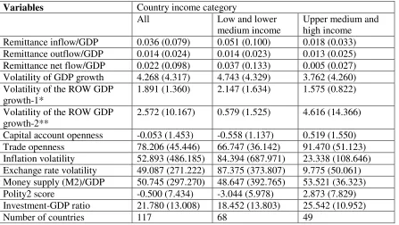
We first provide a brief discussion of the descriptive statistics of the variables

used in the regressions. The results are presented in Table 1.

Insert Table 1 here

The average remittance inflows are about 4% of GDP over the sample period. They are

higher in low (and lower-medium) income countries (above 5%) than in (upper-medium

and) rich countries (less than 2%). The average remittance outflows, on the other hand,

are less than 1.5% of GDP. This result is conceivable given that remittances usually flow

from high to low income countries. Average growth volatility is higher in low compared

to high income countries. The ROW volatility for home countries is about 1.4 times

larger for low compared to high income countries. Conversely, the ROW volatility for

host countries is about 8 times larger for high than low income countries. In high income

(15)

14 volatile, the ratio of M2 to GDP is higher and institutional quality is better compared to

low income countries.

4.1 Determinants of remittance inflows

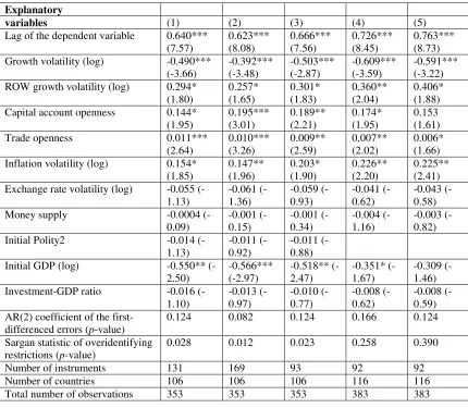
Now we turn to the regression results. The results for the determinants of

remittance inflows for the full sample are presented in Table 2. In column 1, trade and

capital account openness are treated as exogenous. In columns 2-5, the model is

estimated treating openness as endogenous. In column 3, only two lags of both dependent

and independent variables are used as instruments. In all cases, the Sargan statistic shows

that the instruments are invalid. Column 4 re-estimates column 3 excluding polity2. This

increases the number of countries as polity2 data are not available for several low income

countries. The instruments are found to be valid and the AR (2) coefficient of the

first-differenced errors is also insignificant suggesting no serial correlation. The

autoregressive coefficient is 0.73. The result that remittance-GDP ratio is decreasing with

growth volatility in the home country suggests a pro-cyclical behavior of remittance

inflows. Remittance inflows decrease by about 6% for a 10% increase in growth

volatility. On the other hand, the ROW volatility (given by equation (1)) is

counter-cyclical; the remittance-GDP ratio increases by about 4% for a 10% increase in volatility

in host countries.9 Migrant workers remit more during economic downturns probably because of greater uncertainty in host countries. Both trade and capital account openness

increase remittance inflows. Remittance inflows are also increasing with inflation

volatility suggesting the altruistic motive of remittance inflows. This is our preferred

model, so we check the robustness by also estimating the model by the two-step system

GMM with the Windmeijer (2005) corrected robust standard errors (column 5). We find

no meaningful change in the results.

Insert Tables 2-4 here

9

(16)

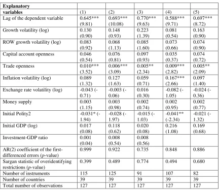
15 We also estimate the model separately for low (and lower-medium) and

(upper-medium and) higher income countries. Table 3 presents results for low income countries.

The number of countries varies between 68 and 73 depending on the choice of

explanatory variables. Columns 1-4 report the results for different combinations of the

explanatory variables and instruments (replication of columns 1-4 in Table 2) but in all

cases the overidentifying restrictions are invalid and the AR (2) coefficient of the

first-differenced errors is significant, so we cast doubt on the validity of the results. In

columns 5 and 6, the model is estimated by the two-step system GMM method; the AR

(2) coefficient remains significant although the instruments are found to be valid.10 The instruments are valid and there is no serial correlation in the errors when the

model is estimated for (upper-medium and) high income countries (Table 4). There are

38 such countries in the sample. We find that growth volatility in the home country does

not affect the remittance inflows but the ROW volatility is negative and significant

suggesting that remittance inflows are pro-cyclical to the ROW volatility. The

remittance-GDP ratio decreases by about 4% when the ROW growth volatility increases

by 10%. Both trade and capital account openness increase remittance inflows. Inflation

volatility contributes positively but its effect is not robust. The ROW volatility becomes

insignificant if the equation is estimated in two steps (column 4). It is also found that the

coefficient of M2-GDP ratio is negative but not robustly significant in the two-step

estimation. It is important to mention that the interest rate differential (M2-GDP ratio is a

proxy for interest rate) between the home and host country is more important for higher

than lower income countries in determining remittance inflows.

The results that ROW volatility is counter-cyclical when both low and high

income countries are combined but pro-cyclical in high income countries implies that

ROW volatility is counter-cyclical in low income countries. We also observe this result in

Table 3 but cannot confirm because of insufficient validity of the model for low income

10

The results are, to a large extent, similar to those for the full sample with the

(17)

16 countries. This is also evident in Figure 2 where we observe that average remittance

inflows to low income countries did not decline during or after the recessions.

4.2 Determinants of remittance outflows

Now we investigate the determinants of remittance outflows. Note that the sample

countries do not match the remittance inflow countries because several countries report

either remittance inflows or outflows.

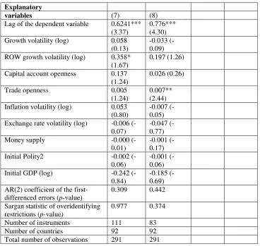
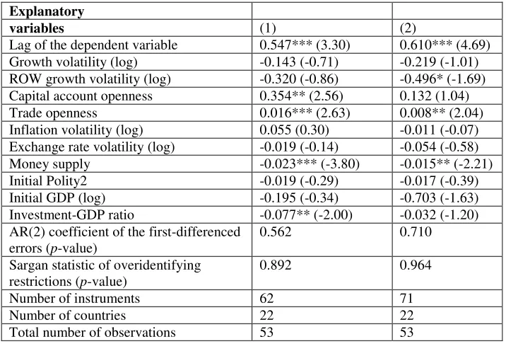
The results for the full sample are presented in Table 5. The ROW volatility for

the host country is now given by equation (2). In columns 1-6, we estimate the model in

one step. The overidentifying restrictions of the instruments are rejected in all cases—

treating the openness measures both as exogenous and endogenous, combinations of

explanatory variables and reducing the number of instruments. However, the instruments

are found to be valid (and no serial correlation of the residual) when the model is

estimated in two steps and excluding the investment-GDP ratio. The autoregressive

coefficient ranges between 0.62 and 0.78 (column 7-8). Other than the lagged dependent

variable, the only two variables found to (positively) affect remittance outflows are the

ROW volatility and trade openness variables although their significance is not robust.

The first result implies that remittance outflows from a host country increase when

volatility in home countries increases suggesting counter-cyclical behavior. For low

income countries, the instruments are also found to be valid only when the model is

estimated in two steps (columns 7-8 in Table 6). For this set of countries, none of the

explanatory variable can explain remittance outflows, even the lagged dependent variable

is weakly significant. This is probably because low income countries are net remittance

recipients.

However, when the model is estimated for high income countries (Table 7), the

instruments are valid and there is no serial correlation in the errors. The autoregressive

coefficient ranges from 0.59 to 0.78 and significant at the 1% level. Trade openness

(18)

17 institutions of the host country are found to reduce remittance outflows. This result

deserves attention, although not robust in all specifications. Migrants save money in a

host country with better institutions probably because they prefer to permanently settle

there.

4.3 Determinants of net remittance flows

Finally, we investigate the determinants of net remittance flows.11

The results for the full sample are presented in Table 8. The overidentifying

restrictions are valid only if two lags of the dependent and independent variables are used

as instruments (columns 3-4 for the one-step and columns 5-6 for the two-step

estimation). Trade openness is again found to be positively and robustly significant. The

important finding is that investment-GDP ratio is negative and significant (although

robustness does not survive in the two-step estimation). The coefficient is around 0.03

suggesting that a 10% increase in investment-GDP ratio reduces net remittance flows by

6.7% (evaluated at the mean value of investment-GDP ratio at 21.78). One possible

explanation is that the investment-GDP ratio is larger in developed countries which also

have a higher capital stock and consequently lower marginal product of capital.

Therefore, a higher investment-GDP ratio attracts lower remittances.

The number of

countries now decreases because, as mentioned earlier, several countries report either

remittance inflows or outflows. We consider only those countries for which net

remittance flows are positive.

The results are also similar when the model is estimated for low income countries

(Table 9). For high income countries, in addition to trade openness, money supply is

negative and significant (Table 10) suggesting that higher interest rates (lower money

supply) attract larger remittance flows to the high income countries. The net flows are

11

(19)

18 counter-cyclical but not robust when trade and capital account openness are treated as

endogenous, and so are capital account openness and investment-GDP ratio.

The above results indicate that remittance inflows are pro-cyclical to home

country volatility. On the other hand, for a host country, remittance outflows are

counter-cyclical to the volatility of home countries. Both results are consistent with the

investment motive in that when volatility in the home country increases, migrants will

remit less money back home. Trade openness is the single most important factor that

increases both remittance inflows and outflows for the home and host countries,

respectively.

5. Concluding remarks

This paper investigates the macroeconomic determinants of remittance inflows

vis-à-vis the role of business cycle fluctuations in host countries. These two important

issues have been ignored in the previous literature. The key innovation of the paper is to

incorporate business cycle information of all host countries by constructing a

rest-of-the-world volatility index for each home country. A separate model for remittance outflows

has been estimated to understand the macroeconomic factors of host countries

responsible for remittance inflows to home countries. The model is estimated by the

dynamic panel system GMM method. The results show that remittance inflows are

pro-cyclical to home country volatility but counter-pro-cyclical to the volatility in host countries.

The above results also hold for low income countries. This result is consistent with the

investment motive. But for high income counties, remittance inflows are acyclical to

home country volatility but pro-cyclical to the volatility in host countries. Trade and

capital account openness increase remittance inflows for both low and high income

countries. On the other hand, for a host country, remittance outflows are counter-cyclical

to the volatility of home countries. This once again is consistent with the investment

motive in that when volatility in the home country increases, migrants will remit less

money back home. Trade openness increases while better institutions decrease remittance

outflows in high income countries. The latter result indicates that migrants remit less if

the host country has better institutions probably because they want to permanently settle

(20)

19 higher interest rates (lower money supply) increases net remittance flows in high income

countries. Trade openness has been found to positively impact on both remittance inflows

and outflows and for both low and high income countries. Lastly, both net remittance

flows and outflows are acyclical to host country volatility.

The results suggest that remittance flows depends on both home and host country

characteristics, and that the macroeconomic determinants cannot be generalized for low

(21)

20 References:

Adams R., and Page J. (2003), “International Migration, Remittances and Poverty in

Developing Countries,” World Bank Policy Research Paper 3179, Washington.

Agarwal R., and Horowitz, A. (2002), “Are International Remittances Altruism or

Insurance? Evidence from Guyana Using Multiple-Migrant Households,” World

Development, 30, 2033-2044.

Akkoyunlu S., and Kholodilin, K. (2008), “A Link between Workers’ Remittances and

Business Cycles in Germany and Turkey,” Emerging Markets, Finance and Trade, 44,

23-40.

Arellano, M., and Bond, S. (1991), “Some Tests of Specification for Panel Data: Monte

Carlo Evidence and an Application to Employment Equations,” Review of Economic

Studies, 58, 277-297.

Arellano, M., and Bover, O. (1995), “Another Look at the Instrumental Variable

Estimation of Error-components Models,” Journal of Econometrics, 68, 29-51.

Bangladesh Bank: http://www.bangladesh-bank.org/.

Beyer, Andreas, and Roger E. A. Farmer (2007), “Natural rate doubts,” Journal of

Economic Dynamics and Control, 31, 797-825.

Blundell, R., and Bond, S. (1998), “Initial Conditions and Moment Restrictions in

Dynamic Panel Data Models,” Journal of Econometrics, 87, 115-143.

Chami R., Hakura, D., and Montiel, P. (2009), “Remittances: An Automatic Output

(22)

21 Chinn, Menzie D., and Ito, Hiro (2008), “A New Measure of Financial Openness,”

Journal of Comparative Policy Analysis, 10 (3, September), 309 – 322.

Cox D., Eser Z., and Jimenez, E. (1998), “Motives for Private Transfers over the Life

Cycle: An Analytical Framework and Evidence for Peru,” Journal of Development

Economics, 55, 57-80.

Giuliano P., and Ruiz-Arranz, M. (2009), “Remittances, Financial Development and

Growth,” Journal of Development Economics, 90, 144-152.

Jackman M., Craigwell, R., and Moore W. (2009), “Economic Volatility and

Remittances: Evidence from SIDS,” Journal of Economic Studies, 36, 135-146.

Kapur D. (2005), “Remittances: the New Development Mantra?” in S. Maimbo and D.

Ratha (eds.) Remittance Development Impact and Future Prospects. World Bank,

Washington.

Koustas, Zisimos, and Apostolos, Serletis (2003), “Long-run Phillips-type trade-offs in

European Union Countries,” Economic Modelling, 20, 679-701.

Lucas R., and Stark, O. (1985), “Motivations to Remit: Evidence from Botswana,”

Journal of Political Economy, 93, 901-918.

Mundaca B. G. (2009), “Remittances, Financial Market Development, and Economic

Growth: The Case of Latin America and the Caribbean,” Review of Development

Economics, 13, 288-2009.

Polity IV Project: Political Regime Characteristics and Transitions, 1800-2007,

(23)

22 Ratha, Dilip, and Shaw, William (2007), “South-South Migration and Remittances,”

Development Prospects Group, World Bank.

Roberts, K., and Morris, M. (2003) “Fortune, Risk and Remittances: An Application of

Option Theory to Participation in Village-Based Migration Networks,” International

Migration Review, 37, 1252-1281.

Sayan, S. (2004), “Guest Workers’ Remittances and Output Fluctuations in Host and

Home Countries: The Case of Remittances from Turkish Workers in Germany,”

Emerging Markets Finance and Trade, 40, 68-81.

Sayan S., and Tekin-Koru, A. (2008), “The Effects of Economic Developments and

Policies in Host Countries on Workers’ Remittance Receipts of Developing Countries:

The Cases of Turkey and Mexico Compared,” in R. Lucas, L. Squire and T. Srinivasan

(eds.), The Impact of Rich Country Policies on Developing Economies. London: Edward

Elgar.

Vargas-Silva, C. (2008), “Are Remittances Manna from Heaven? A Look at the Business

Cycle Properties of Remittances,” North American Journal of Economics and Finance,

19, 290–303.

Windmeijer, F. (2005), “A Finite Sample Correction for the Variance of Linear two-Step

GMM Estimators,” Journal of Econometrics, 126, 25–51.

World Bank (2009):

(24)

[image:24.612.92.539.156.408.2]

23 Tables

Table 1: Descriptive Statistics

Variables Country income category

All Low and lower medium income

Upper medium and high income Remittance inflow/GDP 0.036 (0.079) 0.051 (0.100) 0.018 (0.033) Remittance outflow/GDP 0.014 (0.024) 0.014 (0.023) 0.013 (0.025) Remittance net flow/GDP 0.022 (0.098) 0.037 (0.133) 0.005 (0.027) Volatility of GDP growth 4.268 (4.317) 4.743 (4.329) 3.762 (4.260) Volatility of the ROW GDP

growth-1*

1.891 (1.360) 2.147 (1.634) 1.575 (0.822)

Volatility of the ROW GDP growth-2**

2.572 (10.167) 0.579 (1.525) 4.616 (14.366)

Capital account openness -0.053 (1.453) -0.558 (1.137) 0.519 (1.550) Trade openness 78.206 (45.446) 66.747 (36.142) 91.470 (51.123) Inflation volatility 52.893 (486.185) 84.394 (687.971) 23.338 (108.646) Exchange rate volatility 49.087 (271.222) 87.375 (373.807) 9.775 (50.061) Money supply (M2)/GDP 50.745 (297.270) 48.647 (392.765) 53.521 (36.323) Polity2 score -0.500 (7.434) -3.044 (5.978) 2.873 (7.829) Investment-GDP ratio 21.780 (13.008) 18.452 (13.803) 25.542 (10.952)

Number of countries 117 68 49

(25)

[image:25.612.109.539.131.506.2]

24 Table 2: Determinants of remittance inflows: Log of remittance inflow/GDP is the dependent variable (system GMM estimation of equation 3)

Explanatory

variables (1) (2) (3) (4) (5) Lag of the dependent variable 0.640***

(7.57) 0.623*** (8.08) 0.666*** (7.56) 0.726*** (8.45) 0.763*** (8.73) Growth volatility (log) -0.490***

(-3.66) -0.392*** (-3.48) -0.503*** (-2.87) -0.609*** (-3.59) -0.591*** (-3.22) ROW growth volatility (log) 0.294*

(1.80) 0.257* (1.65) 0.301* (1.83) 0.360** (2.04) 0.406* (1.88) Capital account openness 0.144*

(1.95) 0.195*** (3.01) 0.189** (2.21) 0.174* (1.95) 0.153 (1.61) Trade openness 0.011***

(2.64) 0.010*** (3.26) 0.009** (2.59) 0.007** (2.02) 0.006* (1.66) Inflation volatility (log) 0.154*

(1.85) 0.147** (1.96) 0.203* (1.90) 0.226** (2.20) 0.225** (2.41) Exchange rate volatility (log) -0.055

(-1.13) -0.061 (-1.36) -0.059 (-0.93) -0.041 (-0.62) -0.043 (-0.58) Money supply -0.0004

(-0.09) -0.001 (-0.15) -0.001 (-0.34) -0.004 (-1.16) -0.003 (-0.82) Initial Polity2 -0.014

(-1.13)

-0.011 (-0.92)

-0.011 (-0.88) Initial GDP (log) -0.550**

(-2.50) -0.566*** (-2.97) -0.518** (-2.47) -0.351* (-1.67) -0.309 (-1.46) Investment-GDP ratio -0.016

(-1.10) -0.013 (-0.97) -0.010 (-0.77) -0.008 (-0.62) -0.008 (-0.59) AR(2) coefficient of the

first-differenced errors (p-value)

0.124 0.082 0.124 0.166 0.124

Sargan statistic of overidentifying restrictions (p-value)

0.028 0.012 0.023 0.258 0.390

Number of instruments 131 169 93 92 92 Number of countries 106 106 106 116 116 Total number of observations 353 353 353 383 383

Figures in the parentheses are Arellano-Bond robust t-statistics. ***, **, and * are significant at 1%, 5%, and 10% level, respectively. All equations contain a constant and time dummies but they are not reported. Column 1: All variables except ROW growth volatility, polity2, trade openness, capital account openness, and initial income are endogenous.

Columns 2-4: All variables except ROW growth volatility, polity2, and initial income are endogenous. Columns 3-4: Only two lags are used as instruments.

Column 5: Replicates column 4 by two-step estimation with Windmeijer (2005) corrected robust t -statistics.

(26)

25 Table 3: Determinants of remittance inflows for low- and lower-medium income

countries: Log of remittance inflow/GDP is the dependent variable (system GMM estimation of equation 3)

Explanatory

variables (1) (2) (3) (4) (5) (6) Lag of the dependent variable 0.610***

(8.66) 0.615*** (9.99) 0.660*** (8.97) 0.650*** (9.22) 0.652*** (5.94) 0.649*** (7.42) Growth volatility (log) -0.476***

(-4.12) -0.346*** (-3.82) -0.384** (-2.40) -0.459*** (-2.85) -0.460 (-0.90) -0.501 (-2.11) ROW growth volatility (log) 0.315*

(1.76) 0.336** (2.00) 0.334** (1.98) 0.346* (1.90) 0.358* (1.73) 0.347* (1.86) Capital account openness 0.209**

(2.07) 0.143* (1.87) 0.135 (1.61) 0.115 (1.27) 0.244** (2.16) 0.150 (1.59) Trade openness 0.011**

(2.35) 0.009** (2.47) 0.010** (2.51) 0.010** (2.39) 0.008 (1.63) 0.009** (2.59) Inflation volatility (log) 0.107

(1.41) 0.086 (1.28) 0.137 (1.36) 0.133 (1.35) 0.097 (0.63) 0.155 (1.34) Exchange rate volatility (log) 0.032

(0.58) 0.039 (0.72) 0.076 (1.09) 0.068 (0.96) 0.009 (0.12) 0.046 (0.41) Money supply 0.007

(0.93) 0.008 (1.21) 0.007 (1.12) 0.006 (1.00) 0.005 (0.59) 0.006 (0.87) Initial Polity2 -0.008

(-0.57) 0.006 (0.43) 0.011 (0.71) -0.010 (-0.42) Initial GDP (log) -0.046

(-0.20) 0.032 (0.17) 0.164 (0.82) 0.134 (0.66) -0.028 (-0.08) 0.035 (0.13) Investment-GDP ratio -0.017

(-1.21) -0.011 (-0.96) -0.011 (-0.89) -0.011 (-0.95) -0.016 (-0.80) -0.011 (-0.77) AR(2) coefficient of the

0.031 0.024 0.022 0.030 0.081 0.043

Sargan statistic of

overidentifying restrictions (p -value)

0.000 0.000 0.000 0.000 1.000 0.922

Number of instruments 131 169 93 92 131 92 Number of countries 68 68 68 73 68 73 Total number of observations 234 234 234 246 234 246

Columns 5 and 6: Replicate columns 1 and 4, respectively, by two-step estimation with Windmeijer (2005) corrected robust t-statistics.

(27)

[image:27.612.109.474.120.495.2]

26 Table 4: Determinants of remittance inflows for upper-medium and high income

countries: Log of remittance inflow/GDP is the dependent variable (system GMM estimation of equation 3)

Explanatory

variables (1) (2) (3) (4) Lag of the dependent variable 0.551***

(7.20) 0.549*** (7.44) 0.606*** (8.50) 0.641*** (6.58) Growth volatility (log) -0.138

(-1.10) -0.151 (-1.15) -0.130 (-0.76) -0.003 (-0.02) ROW growth volatility (log) -0.356*

(-1.89) -0.344* (-1.76) -0.355* (-1.71) -0.276 (-1.23) Capital account openness 0.096

(1.31) 0.142** (2.26) 0.207*** (2.76) 0.204* (1.65) Trade openness 0.011***

(3.11) 0.011*** (5.06) 0.011*** (4.02) 0.011** (2.38) Inflation volatility (log) 0.140*

(1.84) 0.119 (1.43) 0.178** (2.01) 0.144 (1.10) Exchange rate volatility (log) -0.095

(-1.25) -0.081 (-1.15) -0.062 (-0.95) -0.102* (-1.92) Money supply -0.005

(-1.46) -0.006* (-1.78) -0.005 (-1.40) -0.006 (-0.96) Initial Polity2 0.021

(0.93) 0.026 (1.11) 0.029 (1.15) 0.048 (1.27) Initial GDP (log) -0.865***

(-2.81) -0.803*** (-2.84) -0.800*** (-2.38) -0.793 (-1.24) Investment-GDP ratio 0.010

(0.55) 0.007 (0.51) 0.002 (0.11) -0.015 (-0.63) AR(2) coefficient of the

0.586 0.570 0.591 0.922

0.849 0.840 0.742 1.00

Number of instruments 109 119 90 90 Number of countries 38 38 38 38 Total number of observations 119 119 119 119

Columns 2-3: All variables except ROW growth volatility, polity2, and initial income are endogenous. Column 3: Only two lags are used as instruments.

(28)

[image:28.612.101.561.132.505.2]

27

Table 5: Determinants of remittance outflows: Log of remittance outflow/GDP is the dependent variable (system GMM estimation of equation 3)

Explanatory

(6.39) 0.691*** (7.58) 0.799*** (7.97) 0.845*** (9.95) 0.628*** (5.17) 0.758*** (5.95) Growth volatility (log) 0.122

(0.98) 0.030 (0.26) 0.061 (0.39) 0.042 (0.29) 0.032 (0.24) -0.013 (-0.07) ROW growth volatility (log) 0.155

(1.19) 0.058 (0.56) 0.063 (0.63) -0.026 (-0.33) 0.366** (2.00) 0.223* (1.65) Capital account openness 0.153**

(2.11) 0.073 (1.30) 0.012 (0.15) 0.009 (0.12) 0.132* (1.70) 0.006 (0.07) Trade openness 0.009***

(3.17) 0.006** (2.41) 0.005* (1.81) 0.003 (1.12) 0.006* (1.82) 0.007*** (2.88) Inflation volatility (log) 0.043

(0.80) 0.069 (1.19) -0.033 (-0.50) -0.028 (-0.42) 0.057 (0.91) -0.029 (-0.38) Exchange rate volatility (log) 0.045

(0.78) 0.048 (1.08) -0.007 (-0.13) -0.034 (-0.73) -0.025 (-0.41) -0.063 (-1.10) Money supply 0.005

(1.26) 0.006 (1.62) 0.004 (1.17) 0.002 (0.93) 0.000 (0.01) -0.001 (-0.33) Initial Polity2 0.008

(0.48) -0.002 (-0.10) 0.010 (0.56) -0.003 (-0.18) -0.001 (-0.04) Initial GDP (log) -0.161

(-0.57) -0.040 (-0.17) -0.068 (-0.32) -0.082 (-0.47) -0.283 (-1.01) -0.175 (-0.89) Investment-GDP ratio -0.023

(-1.28) -0.017 (-1.17) -0.015 (-1.01) -0.011 (-0.90) AR(2) coefficient of the

0.202 0.219 0.210 0.290 0.303 0.369

0.001 0.008 0.002 0.009 0.001 0.002

(29)

28 Table 5 (continued): Determinants of remittance outflows: Log of remittance

outflow/GDP is the dependent variable (system GMM estimation of equation 3)

Explanatory

variables (7) (8) Lag of the dependent variable 0.6241***

(3.37)

0.776*** (4.30) Growth volatility (log) 0.058

(0.13)

-0.033 (-0.09) ROW growth volatility (log) 0.358*

(1.67)

0.197 (1.26)

Capital account openness 0.137 (1.24)

0.026 (0.26)

Trade openness 0.005 (1.24)

0.007** (2.44) Inflation volatility (log) 0.053

(0.80)

-0.007 (-0.05) Exchange rate volatility (log) -0.006

(-0.07)

-0.047 (-0.77) Money supply -0.000

(-0.01)

-0.001 (-0.17) Initial Polity2 -0.002

(-0.06)

-0.001 (-0.06) Initial GDP (log) -0.242

(-0.84)

-0.185 (-0.69) AR(2) coefficient of the

0.309 0.442

0.977 0.374

Number of instruments 111 83 Number of countries 92 92 Total number of observations 291 291

Columns 5 and 6 replicate columns 1 and 3, respectively, but exclude investment-output ratio.

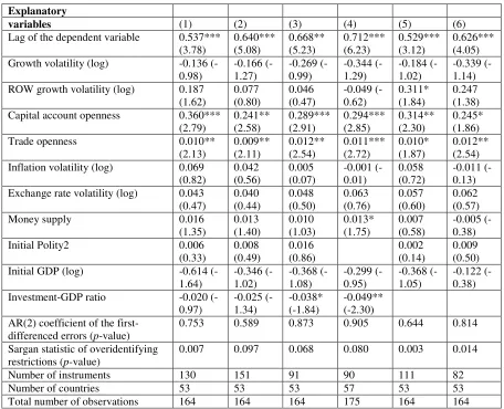
[image:29.612.100.468.106.455.2]

(30)

29 Table 6: Determinants of remittance outflows for low- and lower medium income

countries: Log of remittance outflow/GDP is the dependent variable (system GMM estimation of equation 3)

Explanatory

(3.78) 0.640*** (5.08) 0.668** (5.23) 0.712*** (6.23) 0.529*** (3.12) 0.626*** (4.05) Growth volatility (log) -0.136

(-0.98) -0.166 (-1.27) -0.269 (-0.99) -0.344 (-1.29) -0.184 (-1.02) -0.339 (-1.14) ROW growth volatility (log) 0.187

(1.62) 0.077 (0.80) 0.046 (0.47) -0.049 (-0.62) 0.311* (1.84) 0.247 (1.38) Capital account openness 0.360***

(2.79) 0.241** (2.58) 0.289*** (2.91) 0.294*** (2.85) 0.314** (2.30) 0.245* (1.86) Trade openness 0.010**

(2.13) 0.009** (2.11) 0.012** (2.54) 0.011*** (2.72) 0.010* (1.87) 0.012** (2.54) Inflation volatility (log) 0.069

(0.82) 0.042 (0.56) 0.005 (0.07) -0.001 (-0.01) 0.058 (0.72) -0.011 (-0.13) Exchange rate volatility (log) 0.043

(0.47) 0.040 (0.44) 0.048 (0.50) 0.063 (0.76) 0.057 (0.60) 0.062 (0.57) Money supply 0.016

(1.35) 0.013 (1.40) 0.010 (1.03) 0.013* (1.75) 0.007 (0.58) -0.005 (-0.38) Initial Polity2 0.006

(0.33) 0.008 (0.49) 0.016 (0.86) 0.002 (0.14) 0.009 (0.50) Initial GDP (log) -0.614

(-1.64) -0.346 (-1.02) -0.368 (-1.08) -0.299 (-0.95) -0.368 (-1.05) -0.122 (-0.38) Investment-GDP ratio -0.020

(-0.97) -0.025 (-1.34) -0.038* (-1.84) -0.049** (-2.30) AR(2) coefficient of the

0.753 0.589 0.873 0.905 0.644 0.814

0.007 0.097 0.068 0.080 0.003 0.014

[image:30.612.92.548.120.490.2]

(31)

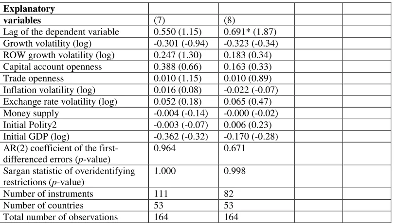
30 Table 6 (continued): Determinants of remittance outflows for low- and lower medium income countries: Log of remittance outflow/GDP is the dependent variable (system GMM estimation of equation 3)

Explanatory

variables (7) (8)

Lag of the dependent variable 0.550 (1.15) 0.691* (1.87) Growth volatility (log) -0.301 (-0.94) -0.323 (-0.34) ROW growth volatility (log) 0.247 (1.30) 0.183 (0.34) Capital account openness 0.388 (0.66) 0.163 (0.33) Trade openness 0.010 (1.15) 0.010 (0.89) Inflation volatility (log) 0.016 (0.08) -0.022 (-0.07) Exchange rate volatility (log) 0.052 (0.18) 0.065 (0.47) Money supply -0.004 (-0.14) -0.000 (-0.02) Initial Polity2 -0.003 (-0.07) 0.006 (0.23) Initial GDP (log) -0.362 (-0.32) -0.170 (-0.28) AR(2) coefficient of the

0.964 0.671

1.000 0.998

Columns 5 and 6 replicate columns 1 and 3, respectively, but exclude investment-output ratio.

[image:31.612.96.504.121.352.2]

(32)

[image:32.612.115.547.118.492.2]

31 Table 7: Determinants of remittance outflows for upper-medium and high income

countries: Log of remittance outflow/GDP is the dependent variable (system GMM estimation of equation 3)

Explanatory

(9.81) 0.693*** (10.08) 0.770*** (9.63) 0.588*** (9.71) 0.697*** (8.72) Growth volatility (log) 0.130

(0.90) 0.148 (0.93) 0.223 (1.39) 0.081 (0.54) 0.163 (0.90) ROW growth volatility (log) 0.083

(0.92) 0.068 (1.13) 0.085 (1.60) 0.073 (0.66) 0.074 (0.90) Capital account openness 0.046

(0.54) 0.076 (0.81) 0.097 (0.93) 0.035 (0.37) 0.074 (0.72) Trade openness 0.010***

(3.52) 0.006*** (3.09) 0.005** (2.34) 0.009*** (2.82) 0.005** (2.09) Inflation volatility (log) 0.089

(1.32) 0.127 (1.63) 0.059 (0.71) 0.167*** (2.66) 0.097 (1.40) Exchange rate volatility (log) -0.043

(-0.71) -0.003 (-0.06) 0.016 (0.30) -0.082 (-1.05) -0.024 (-0.36) Money supply 0.003

(1.15) 0.003 (0.98) 0.002 (0.74) 0.002 (0.95) 0.002 (0.77) Initial Polity2 -0.031*

(-1.94) -0.028 (-1.97) -0.015 (-1.03) -0.041** (-2.34) -0.021 (-1.32) Initial GDP (log) 0.017

(0.08) 0.118 (0.62) 0.020 (0.08) 0.216 (1.08) 0.169 (0.68) Investment-GDP ratio 0.001

(0.04)

0.008 (0.54)

0.008 (0.56) AR(2) coefficient of the

0.999 0.922 0.735 0.848 0.886

0.399 0.489 0.774 0.494 0.680

Columns 2-3: All variables except ROW growth volatility, polity2, and initial income are endogenous. Column 3: Only two lags are used as instruments.

(33)

[image:33.612.94.542.129.503.2]

32 Table 8: Determinants of net remittance flows: Log of net remittance flow/GDP is the dependent variable (system GMM estimation of equation 3)

Explanatory

(5.30) 0.550*** (5.70) 0.597*** (5.31) 0.602*** (5.77) 0.621*** (2.83) 0.609*** (3.47) Growth volatility (log) 0.046

(0.30) 0.056 (0.38) -0.086 (-0.38) 0.007 (0.03) -0.050 (-0.04) -0.055 (-0.05) ROW growth volatility (log) 0.039

(0.12) 0.054 (0.18) 0.037 (0.12) -0.018 (-0.07) 0.070 (0.21) -0.051 (-0.16) Capital account openness 0.202

(1.58) 0.160 (1.49) 0.099 (0.94) 0.104 (0.96) 0.106 (0.63) 0.143 (0.55) Trade openness 0.010*

(1.85) 0.011** (2.41) 0.009** (2.13) 0.007* (1.90) 0.008* (1.68) 0.008 (1.10) Inflation volatility (log) 0.056

(0.50) 0.019 (0.19) 0.031 (0.29) -0.034 (-0.35) 0.067 (0.26) 0.007 (0.03) Exchange rate volatility (log) -0.032

(-0.47) -0.050 (-0.79) -0.034 (-0.48) -0.042 (-0.59) -0.056 (-0.24) -0.047 (-0.17) Money supply -0.004

(-0.60) -0.006 (-0.87) -0.003 (-0.51) -0.007 (-1.07) -0.005 (-0.70) -0.008 (-0.70) Initial Polity2 -0.036*

(-1.67) -0.029 (-1.41) -0.025 (-1.16) -0.031 (-0.66) Initial GDP (log) -0.416

(-1.37) -0.373 (-1.51) -0.383 (-1.57) -0.489** (-2.25) -0.312 (-0.51) -0.474* (-1.98) Investment-GDP ratio -0.035*

(-1.94) -0.035** (-1.99) -0.033** (-2.10) -0.030** (-2.05) -0.029 (-1.29) -0.028 (-1.26) AR(2) coefficient of the

0.414 0.428 0.680 0.937 0.776 0.999

0.089 0.040 0.212 0.120 0.993 0.977

(34)

33 Table 9: Determinants of net remittance flows for low- and lower medium income

countries: Log of net remittance flow/GDP is the dependent variable (system GMM estimation of equation 3)

Explanatory

(5.99) 0.509*** (6.91) 0.479*** (5.78) 0.490*** (5.76) 0.469 (1.54) Growth volatility (log) 0.192

(1.25) 0.186 (1.18) 0.123 (0.61) 0.036 (0.19) -0.056 (-0.08) ROW growth volatility (log) 0.275

(1.05) 0.298 (1.28) 0.279 (1.27) 0.282 (1.25) 0.226 (0.49) Capital account openness 0.298*

(1.82) 0.157 (1.52) 0.137 (1.22) 0.094 (0.93) 0.157 (0.76) Trade openness 0.013**

(2.58) 0.010*** (2.95) 0.012*** (3.46) 0.011** (2.62) 0.011 (1.56) Inflation volatility (log) -0.041

(-0.39) -0.047 (-0.45) -0.091 (-0.86) -0.090 (-0.95) -0.050 (-0.21) Exchange rate volatility (log) 0.012

(0.18) 0.008 (0.14) 0.019 (0.35) -0.035 (-0.61) -0.051 (-0.29) Money supply 0.011

(1.08) 0.007 (0.90) 0.010 (1.12) 0.006 (0.92) 0.008 (0.51) Initial Polity2 -0.008

(-0.33)

0.007 (0.26)

0.015 (0.50) Initial GDP (log) 0.098

(0.41) 0.164 (0.95) 0.116 (0.59) 0.125 (0.62) 0.065 (0.17) Investment-GDP ratio -0.052**

(-2.01) -0.04* (-1.88) -0.044** (-2.29) -0.042** (-2.35) -0.044*** (-3.01) AR(2) coefficient of the

0.647 0.617 0.605 0.861 0.935

0.077 0.104 0.140 0.069 0.999

(35)

[image:35.612.114.472.122.365.2]

34 Table 10: Determinants of net remittance flows for upper-medium and high income countries: Log of net remittance flow/GDP is the dependent variable (system GMM estimation of equation 3)

Explanatory

variables (1) (2)

Lag of the dependent variable 0.547*** (3.30) 0.610*** (4.69) Growth volatility (log) -0.143 (-0.71) -0.219 (-1.01) ROW growth volatility (log) -0.320 (-0.86) -0.496* (-1.69) Capital account openness 0.354** (2.56) 0.132 (1.04) Trade openness 0.016*** (2.63) 0.008** (2.04) Inflation volatility (log) 0.055 (0.30) -0.011 (-0.07) Exchange rate volatility (log) -0.019 (-0.14) -0.054 (-0.58) Money supply -0.023*** (-3.80) -0.015** (-2.21) Initial Polity2 -0.019 (-0.29) -0.017 (-0.39) Initial GDP (log) -0.195 (-0.34) -0.703 (-1.63) Investment-GDP ratio -0.077** (-2.00) -0.032 (-1.20) AR(2) coefficient of the first-differenced

errors (p-value)

0.562 0.710

0.892 0.964

Column 2: All variables except ROW growth volatility, polity2, and initial income are endogenous. Only two lags are used as instruments.

(36)

[image:36.612.116.465.142.363.2]

35 Figures

Figure 1: Average remittance inflows (1970=100)

0

50

0

10

00

15

00

20

00

[image:36.612.113.472.443.648.2]

1970 1980 1990 2000 2010

Figure 2: Average remittance inflows to low and lower-medium income countries (1970=100)

0

10

00

20

00

30

00

40

00

50

00

1970 1980 1990 2000 2010

(37)

[image:37.612.112.463.122.337.2]

36 Figure 3: Average remittance inflows to high-income countries (1970=100)

0

20

0

40

0

60

0

80

0

10

00

1970 1980 1990 2000 2010

Figure 4: Average remittance inflows to upper-medium and high-income countries (1970=100)

0

50

0

10

00

15

00

[image:37.612.111.467.413.648.2]

(38)

37 Appendix:

Variables Data source

Remittance flows World Bank

Real GDP Penn World Table 6.2

Investment-GDP ratio Penn World Table 6.2

Openness (X + M as a % GDP) World Bank

Nominal exchange rate World Bank

M2-GDP ratio World Bank

CPI inflation World Bank

Capital account openness Chinn and Ito (2008)

Polity2 Polity IV Project: Political Regime