I feel good! Gender differences and reporting heterogeneity in self assessed health

Munich Personal RePEc Archive

I feel good! Gender differences and

reporting heterogeneity in self-assessed

health

Pfarr, Christian and Schneider, Brit S. and Schneider, Udo

and Ulrich, Volker

University of Bayreuth

3 August 2010

Online at

https://mpra.ub.uni-muenchen.de/24231/

I feel good!

Gender differences and reporting

heterogeneity in self-assessed health

Christian Pfarr, Brit S. Schneider, Udo Schneider, Volker Ulrich

University of Bayreuth, Department of Law and Economics

Institute of Public Finance

Bayreuth, Germany

+49-921-552929

+49-921-55842929

udo.schneider@uni-bayreuth.de

http://www.fiwi.uni-bayreuth.de

For empirical analysis and policy-oriented recommendation, the precise measurement of individual

health or well-being is essential. The problem with variables based on questionnaires such as

self-assessed health is that the answer may depend on individual reporting behaviour. Moreover, if

individual‟s health perception varies with certain attitudes of the respondent reporting heterogene i-ty may lead to index or cut-point shifts of the health distribution, causing estimation problems. We

analyse the reporting behaviour of individuals on their self-assessed health status, a five-point

categorical variable. We explore observed heterogeneity in categorical variables and include

unob-served individual heterogeneity using German panel data. Estimation results show different

im-pacts of socioeconomic and health related variables on the five subscales of self-assessed health.

Moreover, the answering behaviour varies between female and male respondents, pointing to

gen-der specific perception and assessment of diseases. Reporting behaviour on self-assessed health

questions in surveys is problematic due to a possible heterogeneity. Hence, in case of reporting

heterogeneity, using self-assessed measures in empirical studies may be misleading or at least

ambiguous.

JEL-Classification: I12, C21

Keywords: reporting heterogeneity, generalized ordered probit, self-assessed

1. Introduction

The measurement of individual health or well-being is crucial in health econom-ics. In many empirical studies, various measures like self-assessed health, satis-faction with health or health worries are used [1, 2]. Such indicators are common to data sets and help to compare the results of different studies. The problem with the use of such variables is that the answer depends on the one hand on the ques-tionnaire or even on the interviewer and on the other hand on the individual per-ception of the question.

In the following, we concentrate on individual reporting behaviour and look for systematic differences between population subgroups. If the reporting behaviour is related to socioeconomic status, age, education or labour force status, different subgroups of the population report their health status differently. Problems arise if self-reported health that is used as explanatory variable is prawn to endogeneity problems. In the empirical analysis, we use data from the German SAVE study where multiple imputation methods are used to deal with item non-response. Be-sides a categorical measure of self-related health several questions about the indi-vidual experience with sever or chronic diseases are included and may serve as objective health status.

Individual answers are the basis to the question about self-assessed health status, a five-point categorical variable. We show that a simple ordered probit analysis neglects the fact that the classification into the five subscales depends on socioec-onomic as well as health related variables. Moreover, the answers differ between female and male respondents. To take care of these problems, we use a general-ized ordered probit estimation to cope with a possible heterogeneity in reporting behaviour and to identify possible sources of heterogeneity. This technique can be used to measure how reliably a person carries out health related items in a ques-tionnaire.

2. Literature review

The literature about the use and interpretation of health indicators like self-assessed health in empirical research is widespread. Among the first, Butler et al. [3] discuss a potential measurement error in self-reported health when studying work behaviour. They analyse the relationship between a dichotomous measure of self-reported health and a clinical indicator. The clinical indicator covered symp-toms of arthritis while self-reported health is based on the question whether the respondent had arthritis or rheumatism. Empirical evidence shows that working individuals correctly report their health more likely. The same results are obtained for high school education and higher income. As a consequence, Butler et al. ar-gue that traditional measures of self-reported health are valid indicators of actual health but have to be used in line with socioeconomic characteristics.

The difference between self-reported and objective measures of health like

specif-ic health conditions or limitations or doctor‟s reports for the retirement decision is

analysed by Bound [4]. He follows that the problem of endogeneity and meas-urement error problems cannot be solved simultaneously. For his analysis, he uses self-reported health and one objective health measure. If the latter is not perfectly correlated with current health status the statistical model is not identified.

The impact of different health measures is analysed using the Retirement History Survey. When self-reported measures are used, health is more important than eco-nomic factors compared to the usage of more objective health measures. Moreo-ver, both measures show a potential bias. As long as the objective proxies are not perfectly correlated with work capacity errors in variables problems occur that lead to a potential bias.

con-clusions. Using Canadian data, Baker et al. [6] find evidence that there exist sub-stantial errors in measures of self-reported health. Moreover, these errors seem to be smaller for those in the labour force while they are larger if the assessment of health leaves room for subjective interpretation. Disney et al. [7] focus on retire-ment behaviour in Britain and the influence of ill health. They use self-assessed health as the predictor of health status and instrument this variable using an or-dered probit model with health indicator variables and personal characteristics as explanatory variables. The predicted values of this model are then normalized and the resulting health stock enters the retirement equation to mitigate a possible en-dogeneity problem.

A review about the relationship between labour force status of older workers and health is presented by Lindeboom [8]. The important influence of health and fi-nancial incentives on the decision to retire is overshadowed by measurement problems and the fact that health and work are jointly determined. He discusses a framework for the interrelations between health and work focussing on the meas-urement of health. If both, subjective and objective indicators of health are only poor measures of that health status that is relevant for work-related decisions this will lead to a downward bias in the effects of health. For empirical models, Lindeboom and Kerkhofs [9] specify a model where the individual differences in reporting can be taken into account by an estimation strategy where the response thresholds of a model for ordered categories depend e.g. on the labour force sta-tus.

report-ing could be ruled out for all countries under review as well as a parallel shift of the reporting thresholds, implying that the assessment of the same health catego-ries will differ between countcatego-ries. Ziebarth [12] presents a comparison of different health measures in case of reporting heterogeneity and analyses their impact on an indicator of inequality (concentration index as a form of inequality measure). He finds that self-assessed health goes along with the highest degree of inequality. If alternatively a variable like doctor visits is used, the concentration index is signif-icantly lower, i.e. it is reduced by the factor ten if the SF-12 health indicator is used. Summarizing, Ziebarth argues that income-related reporting heterogeneity is a complex problem in generic health measures.

Another strand of the literature [13] analyses the presence of cut-point and index shifts in self-reported health measures. Heterogeneous reporting behaviour means that different population sub-groups use different reference points when answer-ing health related questions. Thereby, an index shift may occur if the reportanswer-ing behaviour leads to a parallel shift of the thresholds while the relative position of the categories remains unchanged. With a cut-point shift, the thresholds are af-fected differently by the response behaviour. Lindeboom et al. find evidence for both kinds of shifts depending on age and gender but not on income, education or language skills.

Effects of different wordings in questionnaires and consequences of reporting bias and heterogeneity are studied by Hernández-Quevedo et al. [14]. They focus on the existence of index and cut-point shifts in the British Household Panel Survey. The change of the questionnaire in wave eight can be interpreted as a natural ex-periment. By applying ordered probit and generalized ordered probit models, they can show that there was an index shift in wave 9 but find no evidence for a cut-point shift due to the different wording in wave 9 questionnaire on self-reported health.

With French data from 2001, the estimation results show that there is substantial income-related heterogeneity in self-assessed health.

From an international perspective, Juerges [16] explores the differences in true vs. reported health using data from the Survey of Health, Ageing and Retirement in Europe for the year 2004. For ten countries, he finds that self-reported health shows large cross-country differences. The variation could be reduced if self-reported health distributions are assumed to possess an underlying identical re-sponse style. This means that cross-country variation depends to a certain amount on the differences in reporting styles.

Our paper can be classified into the literature as follows: we analyse the reporting behaviour of individuals to questions on their self-assessed health status by esti-mating random effects generalized ordered probit models that allow deviating from the parallel regression assumption. In other words, the individual assessment

“good or bad health” can be found to be fundamentally different dependent on

individuals´ socioeconomic characteristics. Moreover, we also test for cut-point shifts in the data, i.e. that the five categories of self-assessed health (very good, good, medium, bad, very bad) are not constant between individuals but may also vary between the observation units.

3. Data and estimation method

For the present analysis, we use date from the German SAVE study.1 Like in other survey studies, item non-response can lead to problems for the analysis especially for the estimation results and covariance structures [17, 49]. One possibility to deal with this problem is to delete all observations with non-responses which re-duces sample size and goes along with a loss of statistical efficiency. In the SAVE data, missing values are estimated using a variant of the iterative multiple imputa-tion procedure [18]. This is a two-step procedure where in the first step the condi-tional distribution of the missing variables is estimated using regression methods on a sample with complete data (see [17] for further details).2 For the second step,

1 _{The SAVE study is conducted by the Mannheim Research Institute for the Economics of Aging}

(MEA) and started the in 2001. Originally, the longitudinal study on households‟ financial beha v-ior focused on savings and old-age provisions but also deals with aspects of health and health behavior [17].

2 _{The dataset distinguishes between core (e. g. financial data) and non-core variables}

a Markov-Chain Monte-Carlo method is used to replace the missing items in the full data set by multiple draws from the estimated conditional distribution. Hence, we can work with five complete datasets where all missings are replaced by im-puted values.3 These datasets differ slightly with respect to the imputed variables and reflect the uncertainty about the true values of the missing attributes. For all datasets, five repetitions are used to generate each imputed dataset. This procedure leads to a gain in the total observations between 10 % for males and 13 % for fe-males.

For the analysis at hand, we use the years 2006-2008. Our dependent variable is the 5-point categorical variable self-assessed health, with 1 indicating a reported health status that is very bad and 5 a very good health status. As explanatory vari-ables, we use socioeconomic characteristics like age, education, relative income position and labour force status. A description of the variables is presented in Ta-ble 1.4

than 6 % whereas those for the non-core variables are much less than 2 % [17]. A subset of the non-core variables is used as conditioning variables or predictors for the current imputation step.

3 _{Only variables on age and gender contain no missing values.}

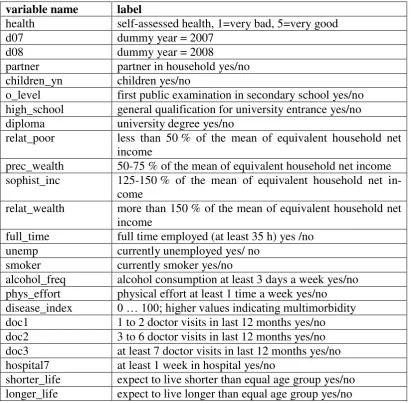
Table 1: Variable description

variable name label

health self-assessed health, 1=very bad, 5=very good

d07 dummy year = 2007

d08 dummy year = 2008

partner partner in household yes/no children_yn children yes/no

o_level first public examination in secondary school yes/no high_school general qualification for university entrance yes/no diploma university degree yes/no

relat_poor less than 50 % of the mean of equivalent household net income

prec_wealth 50-75 % of the mean of equivalent household net income sophist_inc 125-150 % of the mean of equivalent household net

in-come

relat_wealth more than 150 % of the mean of equivalent household net income

full_time full time employed (at least 35 h) yes /no unemp currently unemployed yes/ no

smoker currently smoker yes/no

alcohol_freq alcohol consumption at least 3 days a week yes/no phys_effort physical effort at least 1 time a week yes/no disease_index 0 … 100; higher values indicating multimorbidity doc1 1 to 2 doctor visits in last 12 months yes/no doc2 3 to 6 doctor visits in last 12 months yes/no doc3 at least 7 doctor visits in last 12 months yes/no hospital7 at least 1 week in hospital yes/no

shorter_life expect to live shorter than equal age group yes/no longer_life expect to live longer than equal age group yes/no

To cover nonlinear age effects, we group males and females into age quintiles.5 The lowest quintile is set up by those individuals aged equal to or less than 38 years for males and 36 years for females. The highest quintile contains respond-ents older than 68 or 67 years, respectively. The detailed thresholds between the quintiles can be obtained from Table 2.

Table 2: Age Variables: average thresholds

variable name male female

age0 <=38 <=36

age1 >38 and <=48 >36 and <=45 age2 >48 and <=58 >45 and <=55 age3 >58 and <=68 >55 and <=67

age4 >68 >67

5 _{The intervals for the quintiles are averaged across years and imputations. Only small differences}

Moreover, health relevant behaviour and experiences with a severe or chronic illness are included in the data set. The latter information is more related to sick-ness than the self-reported health but still a subjective measure. According to Kerkhofs and Lindeboom [5], we try to objectify this illness reporting. To

con-struct our disease index, we make use of the binary variable “health problems”

and regress this variable on a set of ten dummy variables indicating various forms of diseases. By doing so, we are able to weight the impact of the different

illness-es on the variable “health problems”. Considering the structure of the dataset, we

run this regression separately for every year and imputation and also for males and females. The prediction of the regression is then transformed to the

continu-ous variable “disease index” ranging from 0 to 100 with mean 50 and a standard

deviation of 10. Furthermore, the use of this objectified variable goes along with more variation in the explanatory variables. Therefore, a higher value of the index indicates a higher degree of multimorbidity. In comparison with the gender-specific average, an above-average index points to more illness-related problems (relatively).

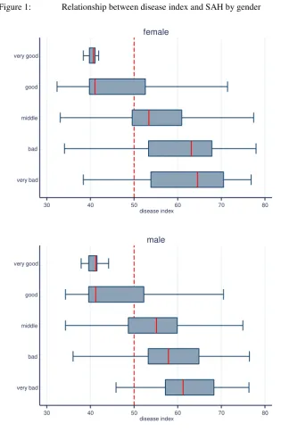
The relation between our constructed index and self-assessed health can be seen from figure 1. It is obvious that a better reported health goes along with a lower value of the disease index for females as well as for males. The shadowed box resembles 50 per cent of the data in the relevant health category. One striking re-sult is that the box for the best health status (very good) is very narrow, which means that there exists only few variation in the values of the disease index. The median is marked by the vertical line within the box. For both genders, in the

cat-egory “good” the median is at the left side of the box, which means the distrib u-tion is skewed. For the two lower health categories, we observe some differences between females and males. First, the 50 % boxes are smaller for men and second, the median of females is on a larger scale. Hence, females show a larger spread of

the disease index within health categories “bad” and “very bad”. With respect to the adjacent lines (whiskers), differences occur for the category “very bad”. Here

Figure 1: Relationship between disease index and SAH by gender

30 40 50 60 70 80

disease index very good

good

middle

bad

very bad

female

30 40 50 60 70 80

disease index very good

good

middle

bad

very bad

male

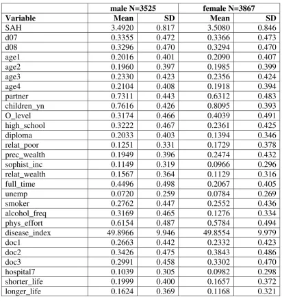
In Table 3, the statistics for the first imputation are presented for males and fe-males.6 As can be seen for self-assessed health, no significant difference can be observed between males and females. Females tend to consume alcohol less fre-quently than males (13 vs. 32 per cent). For the highest education level, we find that high school and university degrees are more frequent among men. The same is true for full time working. With respect to income, we use four different dum-my variables to illustrate the relative income position of a household member [19]. For age quintiles, the panel summary statistics shows a deviation from 20 %

because we use a balanced panel and average thresholds vary between the obser-vation years.

Table 3: Summary statistics (imputation 1)

male N=3525 female N=3867

Variable Mean SD Mean SD

SAH 3.4920 0.817 3.5080 0.846

d07 0.3355 0.472 0.3366 0.473

d08 0.3296 0.470 0.3294 0.470

age1 0.2016 0.401 0.2090 0.407

age2 0.1960 0.397 0.1985 0.399

age3 0.2330 0.423 0.2356 0.424

age4 0.2104 0.408 0.1918 0.394

partner 0.7311 0.443 0.6312 0.483

children_yn 0.7616 0.426 0.8095 0.393

O_level 0.3174 0.466 0.4039 0.491

high_school 0.3222 0.467 0.2361 0.425

diploma 0.2033 0.403 0.1394 0.346

relat_poor 0.1251 0.331 0.1729 0.378

prec_wealth 0.1949 0.396 0.2474 0.432

sophist_inc 0.1149 0.319 0.0966 0.296

relat_wealth 0.1567 0.364 0.1129 0.316

full_time 0.4496 0.498 0.2067 0.405

unemp 0.0720 0.259 0.0784 0.269

smoker 0.2762 0.447 0.2552 0.436

alcohol_freq 0.3169 0.465 0.1276 0.334

phys_effort 0.6154 0.487 0.5784 0.494

disease_index 49.8966 9.946 49.8554 9.979

doc1 0.2663 0.442 0.2332 0.423

doc2 0.3426 0.475 0.3843 0.486

doc3 0.2991 0.458 0.3302 0.470

hospital7 0.1039 0.305 0.0982 0.298

shorter_life 0.1999 0.400 0.1657 0.372

longer_life 0.1624 0.369 0.1168 0.321

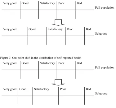
Index shift and cut-point shift

situation where reporting of the full population is compared to the reporting of a subgroup [14]. The differences between both forms of reporting heterogeneity can be seen from figures 2 and 3.

Figure 2: Index shift in the distribution of self-reported health

Very good Good Satisfactory Poor Bad

Full population

Very good Good Satisfactory Poor Bad

Subgroup

Figure 3: Cut-point shift in the distribution of self-reported health

Very good Good Satisfactory Poor Bad

Full population

Very good Good Satisfactory Poor Bad

Subgroup

Source: [14].

An index shift may occur when switching from the full population to a subgroup. One example is when in a specific cultural group all individuals are more reserved about their health evaluation [13]. An example for a cut-point shift is if the cultur-al subgroup is self-conscious about the sentence's wording in the questionnaire and if this leads to a change in the relative position of the categories e. g. in the

threshold for the category „very good‟.8

7 _{Hernández-Quevedo et al. [14] argue that the term „index shift‟ is misleading. Instead, they state}

that the parallel shift in the distribution may be due to a cut-point shift or due to a shift in the un-derlying measure of true health, i. e. the latent variable.

8

Estimation approach9

The variable self-assessed health is a five-point categorical variable. Underlying this observed variable is the latent health status of the respondent y*. In this case, ordered response models are the standard estimation procedure. Following the presentation in Boes and Winkelmann [21] and focusing on the cross-section case first, let y be the ordered categorical outcome, y  {1, 2,…, J}. J denotes the number of distinct categories. The cumulative probabilities of the discrete out-come are then related to a set of explanatory variables x:









Pr       

(1)

Here, j are the unknown threshold parameters and s are the unknown coeffi-cients.10 The function F is often replaced by a standard normal or logistic distribu-tion. In the first case, an ordered probit model results, the second case is an or-dered logit model. Including the underlying latent variable one gets:

J j

u x y j

y if andonly if _j1 *  _j 1,,

This means that the thresholds divide the real line (y*) into J categories. Moreo-ver, observable and unobservable factors influence the latent variable health. For the latter factors, a zero mean and a constant variance is assumed, e.g. 2 = 1 for the ordered probit model.

The probability that a respondent reports his health status to be in category j can then be written as:







 



(2)

For identification purposes, it is necessary to set the constant of the regression to zero and to assume a constant variance. One obstacle to the ordered probit model is the single index or parallel regression assumption [22]. From equation (1) it follows that the coefficient vector  is the same for all categories j. This means that with the increase of an independent variable, the cumulated distribution shifts

assume that a parallel shift in the thresholds that is common to all respondents can be viewed as the simplest form of an index shift. While testing for an index shift is possible in ordered response models like ordered probit, the test of a cut-point shift is implemented using a generalized ordered probit model that allows the parameter to vary between the different categories of the reported health variable.

9 _{Greene and Hensher [20] discuss aspects of heterogeneity in ordered choices and present a}

to the right or left but there is no shift in the slope of the distribution. Hence, one can compare an ordered response model to one in which a set of binary response models with different intercepts is estimated. Such a change in the intercept leads to a shift in the probability curve but leaves the slope unchanged. Relaxing this assumption and allowing the indices to differ across the outcomes leads to the generalized ordered probit model. Here, the threshold parameters depend on the covariates:

j j

j  x

 ~

,

where j are the influence parameters of the covariates on the thresholds. Entering the threshold equation above into the cumulative probability of the generalized ordered probit model leads to the following expression:







 



Pr             

(3)

As one can see from equation (3), the coefficients of the covariates and the threshold coefficients cannot be identified separately when the same set of varia-bles x is used. Hence, it follows that j =  – j and that the generalized ordered probit model has one index x’βjfor each category j of the outcome variable.11 This approach leads to the estimation of J-1 binary probit models [23]. The first model estimates category 1 versus categories 2,.., J; the second model categories 1 and 2 versus 3,.., J. Equation J-1 then compares the choice between categories 1,.., J-1 versus category J. This specification allows for individual heterogeneity in the  -parameters that leads to heterogeneity across the categories of the dependent vari-able.

For our panel data, we use a random effects generalized ordered probit approach [24]. More formally, let SAH be an ordinal variable which takes on the values y =

1, …, J. For the data at hand, i denotes the cross-sectional unit and t the time di-mension. In contrast to the cross-section representation, the outcome probabilities are conditional on the individual effect i:

10 _{One assumption on the threshold parameters is that }

j > j-1, j and that J =  and 0 = -. 11 _{The generalized ordered probit model nests the standard ordered probit model with the}















 











| , 2, , 1

| , 1

it it i it i

it it i it y i it y i

it it i it J i

P y x F x

P y y x F x F x y J

P y J x F x

                               (4)

For the individual effects, a zero mean and a constant variance ² is assumed so that =²/ (1+²). As for the cross-section version of the generalized ordered pro-bit model, the approach allows several of the y to vary across the categories. Therefore, using panel data allows for the inclusion of two kinds of heterogeneity. First, unobserved individual heterogeneity is captured by our random effects spec-ification of the ordered probit model. Second, differences in the cut-points and therefore in the beta coefficients represent the observed heterogeneity in the re-porting of the self-assessed health variable.

For the estimation of the random effects generalized ordered probit model, we combine an iterative procedure proposed by Williams [23] with the random ef-fects estimation command regoprob by Boes [24].12 _{First, a totally unconstraint} model (all coefficients varying) is estimated. Then we apply Wald tests on each variable to prove whether the coefficients differ across equations. The least signif-icant variable is then constraint to have equal effects, and the model is refitted with constraints and the process is repeated as long as no more insignificant vari-ables result. Moreover, a global Wald test on the full model with constraints is applied that confirms the null hypothesis that the parallel regression assumption is not violated.13

4. Results

Tables 4 and 5 present selected results from our estimation for males and females. The full estimation results containing constraint and unconstraint coefficients are shown in the appendix. We outline key results for those variables for which the parallel regression assumption is rejected. For these variables, we can conclude

12 _{A complete description of the procedure can be found in Pfarr et al. [25]. The related}

user-written Stata program regoprob2 is available at the SSC archive.

13_{The estimation with different imputations requires some caution with respect to the „averaging‟}

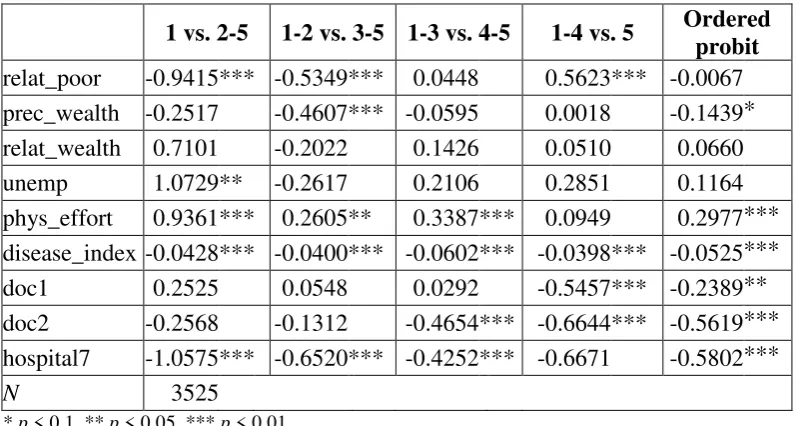
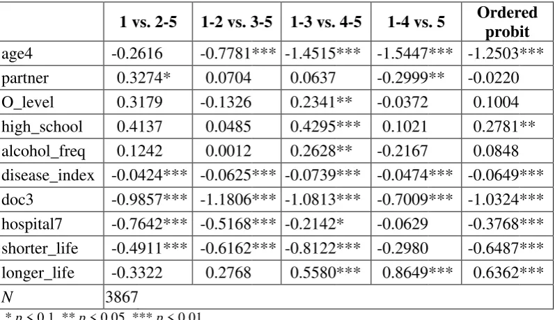
esti-the presence of a cut-point shift leading to esti-the observed heterogeneity of SAH. In the tables, we display the results of two types of estimations. The last column con-tains the ordered probit estimation and the other four columns show the results for the generalized ordered probit model. The latter consists of four binary models. As stated above, the first model estimates category 1 versus categories 2,.., 5 the second model categories 1 and 2 versus 3,.., 5 and so on. If an explanatory factor is included in tables 4 and 5 the coefficients are varying between the categories. This means that these variables are then responsible for a cut-point shift in the distribution of SAH and therefore cause the observed heterogeneity.

One main finding from the generalized ordered probit is that observed heterogene-ity of SAH is caused by different variables for males and females. Explanatory variables are classified in income-related, socio-economic, and health-related fac-tors. Health-related variables (smoking, alcohol consumption, disease index, doc-tor visits) vary between categories for males and females whereas income varia-tion is only found for males and the socio-economic factors (age, educavaria-tion) drive the observed heterogeneity in health reporting for females. One has to emphasise that all explanatory variables enter the estimation but the variables given in tables 4 and 5 drive the observed heterogeneity.

Table 4: Combined selected results generalized ordered probit and ordered probit; males

1 vs. 2-5 1-2 vs. 3-5 1-3 vs. 4-5 1-4 vs. 5 Ordered probit

relat_poor -0.9415 *** -0.5349 *** 0.0448 0.5623 *** -0.0067 prec_wealth -0.2517 -0.4607 *** -0.0595 0.0018 -0.1439 * relat_wealth 0.7101 -0.2022 0.1426 0.0510 0.0660 unemp 1.0729 ** -0.2617 0.2106 0.2851 0.1164 phys_effort 0.9361 *** 0.2605 ** 0.3387 *** 0.0949 0.2977 *** disease_index -0.0428 *** -0.0400 *** -0.0602 *** -0.0398 *** -0.0525 *** doc1 0.2525 0.0548 0.0292 -0.5457 *** -0.2389 ** doc2 -0.2568 -0.1312 -0.4654 *** -0.6644 *** -0.5619 *** hospital7 -1.0575 *** -0.6520 *** -0.4252 *** -0.6671 -0.5802 ***

N 3525

* p < 0.1, ** p < 0.05, *** p < 0.01

Table 5: Combined selected results generalized ordered probit and ordered probit; females

1 vs. 2-5 1-2 vs. 3-5 1-3 vs. 4-5 1-4 vs. 5 Ordered probit

age4 -0.2616 -0.7781 *** -1.4515 *** -1.5447 *** -1.2503 *** partner 0.3274 * 0.0704 0.0637 -0.2999 ** -0.0220 O_level 0.3179 -0.1326 0.2341 ** -0.0372 0.1004 high_school 0.4137 0.0485 0.4295 *** 0.1021 0.2781 ** alcohol_freq 0.1242 0.0012 0.2628 ** -0.2167 0.0848 disease_index -0.0424 *** -0.0625 *** -0.0739 *** -0.0474 *** -0.0649 *** doc3 -0.9857 *** -1.1806 *** -1.0813 *** -0.7009 *** -1.0324 *** hospital7 -0.7642 *** -0.5168 *** -0.2142 * -0.0629 -0.3768 *** shorter_life -0.4911 *** -0.6162 *** -0.8122 *** -0.2980 -0.6487 *** longer_life -0.3322 0.2768 0.5580 *** 0.8649 *** 0.6362 ***

N 3867

* p < 0.1, ** p < 0.05, *** p < 0.01

In a simple ordered probit estimation, the impact of income on SAH is weak or not significant for males. In contrast, generalized ordered probit estimates show that individual health varies with income. In more detail, relative poor individuals tend to report a very bad or bad health status more often. Surprisingly, for the highest health status (1-4 vs. 5) we derive a positive effect of relative poverty on SAH, e.g. fighting poverty is important for but not identical to improving health. Moreover, the constraint variable precarious wealth goes along with a significant-ly negative effect on the reported health level. In addition, the impact of relative wealth is significantly positive. In the female estimation, all the income variables are constraint.

Within the group of variables causing heterogeneity for females, education (O-level and high school) is only significantly positive for those in satisfactory health conditions (categories 1-3 vs. 4-5). Standard ordered probit estimation shows no significant impact for O-level. Compared to women with a rather low knowledge stock, the positive influence of education on SAH implies that the probability of being in a good health status increases with better education. The ordered probit model for women shows no significance for a university degree; this is the only training variable with significance in the male sample.

sport lowers the probability for reporting a bad health status significantly while the effect on the highest health category is insignificant. Sport may generate health benefits: through direct participation as well as communication, educational benefits and social mobilization. Because physical inactivity is a primary risk for chronic diseases, sports can play a critical role in slowing the spread of chronic diseases, reducing their social and economic burden, and saving lives. But not to be forgotten sports has also the potential for damaging health. Athletic injuries or other health problems relate directly to physical activity. All in all the impact of sports on health remains indefinite.

As regards health care utilisation (doctor visits), one would expect that 1 or 2 doc-tor visits in the last year have little impact on individual health status because the-se few visits have more or less preventive character. This view of health care de-mand is rejected for males. While the ordered probit model suggests a significant negative impact, the generalized model shows a negative effect only for the best health status (1-4 vs. 5). For the health effect of just a few doctor visits, one can-not give a clear-cut answer. Regarding 3-6 visits (doc2), we find a significantly negative influence for the two upper categories of SAH. Having more than 6 doc-tor visits in the last twelve months (doc3) has the expected negative sign for all categories but is only varying throughout the categories for females. Another key result is that reporting heterogeneity is found for doctor visits but with gender-specific characteristics.

Our disease index is varying for both males and females. All effects are highly significant and negative. They are strongest when comparing categories 1-3 with 4-5 resulting in a tendency to report a health status satisfactory or lower. This re-sults in a grouping of categories 1-3 and 4-5. This means that health problems caused by different forms of illnesses and consequently multimorbidity leads to reporting heterogeneity. Subsequently, comparing illness-related questions and questions on self-assessed health leads to the conclusion that heterogeneity is driven by disease experiences.

To sum up, the estimation of a generalized ordered probit strongly suggest that there is a cut-point shift in the distribution of self-assessed health.14 Moreover, our

14

estimations provide evidence that the variables causing observed heterogeneity in health status differ notably between males and females. As the generalized or-dered probit estimation points out, income-related, socio-economic, and health-related factors suggest that reporting heterogeneity should be taken into account. As a consequence, caution is necessary when using self-reported measures of health in empirical studies. Moreover, the results also suggest that the influence of the factors above should be considered when designing questionnaires.

5. Conclusion

How reliable are individual answers about self-assessed health? A lot of empirical studies use self-assessed health as qualitative five-point categorical variable on the left hand side of ordered probit models. In the paper, we express doubts that a random effects ordered probit model is a suitable approach for analysing determi-nants of self-assessed health. This model neglects the fact that the classification into the five subscales depends on socioeconomic as well as health related varia-bles. Moreover, the answering behaviour differs between female and male re-spondents. The results of a random effects generalized ordered probit estimation help on the one hand to detect a possible heterogeneity in reporting behaviour and on the other hand to identify possible sources of heterogeneity. In contrast to a random effects ordered probit estimation, our approach combines the detection of observed heterogeneity in categorical variables with the inclusion of unobserved individual heterogeneity using panel data.

Our research contributes to the diversified literature on a possible reporting bias in self-assessed health. Unlike studies on labour force participation or income ine-quality, we do not focus on reporting behaviour in a special case. Instead, we try to show that heterogeneity may depend on gender-specific variables. Among oth-ers, experience with different kinds of illnesses may be one source of different reporting behaviour. Income as a possible source of heterogeneity is more im-portant for men than for women. Other gender differences exist with respect to the influence of education on the reporting behaviour of health. Our estimation ap-proach helps to detect how socioeconomic determinants and health experiences differently influence the individual reporting behaviour.

Hence, our evidence relates to the question how reliably a person completes health related items in a questionnaire. Generally spoken, evaluating question-naires from panel data based on population subgroups such as migrants, children, older people or questionnaires from different countries run the risk to compare apples and oranges if the problem of reporting heterogeneity is not adequately taken into account. Especially the results of the disease index indicate that indi-vidual experiences in the past drive the answering behaviour. Thus, to control for heterogeneous responses to the SAH question it is required to include individual illness episodes in the questionnaire. Using such information is important to as-sess the correct health status but this information has to be weighted in order to retrieve an objectified measure of health. Otherwise, one would explain the heter-ogeneity of self-assessed health with the subjective illness perception.

Our findings show that a widespread and common measure of health like SAH is prone to heterogeneity and that objectified health indicators can be used to detect this bias.

For further research, it would be interesting to evaluate different approaches to objectify additional health indicators. One way may be to capture the effects of

partner‟s health status and disease experience on the reporting of health. With

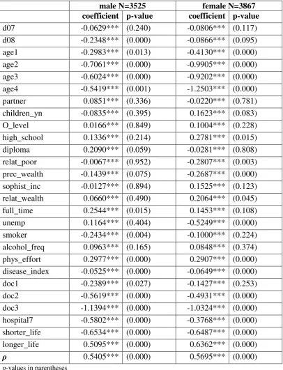
6. Appendix

Table 1: Random effects ordered probit estimates

male N=3525 female N=3867

coefficient p-value coefficient p-value

d07 -0.0629*** (0.240) -0.0806*** (0.117)

d08 -0.2348*** (0.000) -0.0866*** (0.095)

age1 -0.2983*** (0.013) -0.4130*** (0.000)

age2 -0.7061*** (0.000) -0.9905*** (0.000)

age3 -0.6024*** (0.000) -0.9202*** (0.000)

age4 -0.5419*** (0.001) -1.2503*** (0.000)

partner 0.0851*** (0.336) -0.0220*** (0.781) children_yn -0.0835*** (0.395) 0.1623*** (0.083) O_level 0.0166*** (0.849) 0.1004*** (0.228) high_school 0.1336*** (0.214) 0.2781*** (0.015) diploma 0.2090*** (0.059) -0.0281*** (0.808) relat_poor -0.0067*** (0.952) -0.2807*** (0.003) prec_wealth -0.1439*** (0.075) -0.2687*** (0.000) sophist_inc -0.0127*** (0.894) 0.1525*** (0.123) relat_wealth 0.0660*** (0.490) 0.2064*** (0.045) full_time 0.2544*** (0.015) 0.1453*** (0.108)

unemp 0.1164*** (0.404) -0.5249*** (0.000)

smoker -0.2434*** (0.004) -0.1000*** (0.224) alcohol_freq 0.0963*** (0.165) 0.0848*** (0.374) phys_effort 0.2977*** (0.000) 0.2907*** (0.000) disease_index -0.0525*** (0.000) -0.0649*** (0.000)

doc1 -0.2389*** (0.027) -0.1427*** (0.253)

doc2 -0.5619*** (0.000) -0.4931*** (0.000)

doc3 -1.1394*** (0.000) -1.0324*** (0.000)

hospital7 -0.5802*** (0.000) -0.3768*** (0.000) shorter_life -0.6534*** (0.000) -0.6487*** (0.000) longer_life 0.5095*** (0.000) 0.6362*** (0.000)

ρ 0.5405*** (0.000) 0.5695*** (0.000)

p-values in parentheses

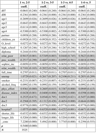
Table 2: Random effects generalized ordered probit males

1 vs. 2-5 1-2 vs. 3-5 1-3 vs. 4-5 1-4 vs. 5

coeff. coeff. coeff. coeff.

d07 -0.0641 (0.240) -0.0641 (0.240) -0.0641 (0.240) -0.0641 (0.240) d08 -0.2361 (0.000) -0.2361 (0.000) -0.2361 (0.000) -0.2361 (0.000) age1 -0.2699 (0.026) -0.2699 (0.026) -0.2699 (0.026) -0.2699 (0.026) age2 -0.6643 (0.000) -0.6643 (0.000) -0.6643 (0.000) -0.6643 (0.000) age3 -0.6114 (0.000) -0.6114 (0.000) -0.6114 (0.000) -0.6114 (0.000) age4 -0.5300 (0.002) -0.5300 (0.002) -0.5300 (0.002) -0.5300 (0.002) partner 0.0958 (0.288) 0.0958 (0.288) 0.0958 (0.288) 0.0958 (0.288) children_yn -0.0928 (0.352) -0.0928 (0.352) -0.0928 (0.352) -0.0928 (0.352) O_level 0.0272 (0.758) 0.0272 (0.758) 0.0272 (0.758) 0.0272 (0.758) high_school 0.1267 (0.246) 0.1267 (0.246) 0.1267 (0.246) 0.1267 (0.246) diploma 0.2444 (0.030) 0.2444 (0.030) 0.2444 (0.030) 0.2444 (0.030) relat_poor -0.9415 (0.001) -0.5349 (0.003) 0.0448 (0.745) 0.5623 (0.001) prec_wealth -0.2517 (0.299) -0.4607 (0.001) -0.0595 (0.561) 0.0018 (0.990) sophist_inc -0.0050 (0.959) -0.0050 (0.959) -0.0050 (0.959) -0.0050 (0.959) relat_wealth 0.7101 (0.103) -0.2022 (0.234) 0.1426 (0.220) 0.0510 (0.752) full_time 0.2707 (0.011) 0.2707 (0.011) 0.2707 (0.011) 0.2707 (0.011) unemp 1.0729 (0.021) -0.2617 (0.207) 0.2106 (0.211) 0.2851 (0.209) smoker -0.2331 (0.007) -0.2331 (0.007) -0.2331 (0.007) -0.2331 (0.007) alcohol_freq 0.0992 (0.159) 0.0992 (0.159) 0.0992 (0.159) 0.0992 (0.159) phys_effort 0.9361 (0.000) 0.2605 (0.015) 0.3387 (0.000) 0.0949 (0.415) disease_index -0.0428 (0.001) -0.0400 (0.000) -0.0602 (0.000) -0.0398 (0.000) doc1 0.2525 (0.672) 0.0548 (0.795) 0.0292 (0.821) -0.5457 (0.000) doc2 -0.2568 (0.395) -0.1312 (0.428) -0.4654 (0.000) -0.6644 (0.000) doc3 -0.9776 (0.000) -0.9776 (0.000) -0.9776 (0.000) -0.9776 (0.000) hospital7 -1.0575 (0.000) -0.6520 (0.000) -0.4252 (0.001) -0.6671 (0.100) shorter_life -0.6532 (0.000) -0.6532 (0.000) -0.6532 (0.000) -0.6532 (0.000) longer_life 0.5204 (0.000) 0.5204 (0.000) 0.5204 (0.000) 0.5204 (0.000) _cons 7.2280 (0.000) 5.4942 (0.000) 3.7745 (0.000) 0.2394 (0.553)

ρ 0.5480 (0.000)

N ₃₅₂₅

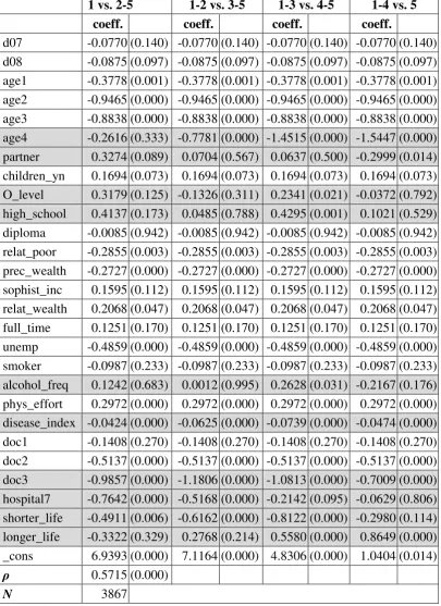
Table 3: Random effects generalized ordered probit females

1 vs. 2-5 1-2 vs. 3-5 1-3 vs. 4-5 1-4 vs. 5

coeff. coeff. coeff. coeff.

d07 -0.0770 (0.140) -0.0770 (0.140) -0.0770 (0.140) -0.0770 (0.140) d08 -0.0875 (0.097) -0.0875 (0.097) -0.0875 (0.097) -0.0875 (0.097) age1 -0.3778 (0.001) -0.3778 (0.001) -0.3778 (0.001) -0.3778 (0.001) age2 -0.9465 (0.000) -0.9465 (0.000) -0.9465 (0.000) -0.9465 (0.000) age3 -0.8838 (0.000) -0.8838 (0.000) -0.8838 (0.000) -0.8838 (0.000) age4 -0.2616 (0.333) -0.7781 (0.000) -1.4515 (0.000) -1.5447 (0.000) partner 0.3274 (0.089) 0.0704 (0.567) 0.0637 (0.500) -0.2999 (0.014) children_yn 0.1694 (0.073) 0.1694 (0.073) 0.1694 (0.073) 0.1694 (0.073) O_level 0.3179 (0.125) -0.1326 (0.311) 0.2341 (0.021) -0.0372 (0.792) high_school 0.4137 (0.173) 0.0485 (0.788) 0.4295 (0.001) 0.1021 (0.529) diploma -0.0085 (0.942) -0.0085 (0.942) -0.0085 (0.942) -0.0085 (0.942) relat_poor -0.2855 (0.003) -0.2855 (0.003) -0.2855 (0.003) -0.2855 (0.003) prec_wealth -0.2727 (0.000) -0.2727 (0.000) -0.2727 (0.000) -0.2727 (0.000) sophist_inc 0.1595 (0.112) 0.1595 (0.112) 0.1595 (0.112) 0.1595 (0.112) relat_wealth 0.2068 (0.047) 0.2068 (0.047) 0.2068 (0.047) 0.2068 (0.047) full_time 0.1251 (0.170) 0.1251 (0.170) 0.1251 (0.170) 0.1251 (0.170) unemp -0.4859 (0.000) -0.4859 (0.000) -0.4859 (0.000) -0.4859 (0.000) smoker -0.0987 (0.233) -0.0987 (0.233) -0.0987 (0.233) -0.0987 (0.233) alcohol_freq 0.1242 (0.683) 0.0012 (0.995) 0.2628 (0.031) -0.2167 (0.176) phys_effort 0.2972 (0.000) 0.2972 (0.000) 0.2972 (0.000) 0.2972 (0.000) disease_index -0.0424 (0.000) -0.0625 (0.000) -0.0739 (0.000) -0.0474 (0.000) doc1 -0.1408 (0.270) -0.1408 (0.270) -0.1408 (0.270) -0.1408 (0.270) doc2 -0.5137 (0.000) -0.5137 (0.000) -0.5137 (0.000) -0.5137 (0.000) doc3 -0.9857 (0.000) -1.1806 (0.000) -1.0813 (0.000) -0.7009 (0.000) hospital7 -0.7642 (0.000) -0.5168 (0.000) -0.2142 (0.095) -0.0629 (0.806) shorter_life -0.4911 (0.006) -0.6162 (0.000) -0.8122 (0.000) -0.2980 (0.114) longer_life -0.3322 (0.329) 0.2768 (0.214) 0.5580 (0.000) 0.8649 (0.000) _cons 6.9393 (0.000) 7.1164 (0.000) 4.8306 (0.000) 1.0404 (0.014)

ρ 0.5715 (0.000)

N ₃₈₆₇

7. Acknowledgements

The authors gratefully acknowledge useful comments from Andreas Schmid, Martin Schellhorn

and participants of the 2010th annual conference in Berlin of the German Association of Health Economics (DGGOE).

8. References

[1] Gerdtham, U., Johannesson, M.: New Estimates of the Demand for Health: Results Based on a

Categorical Health Measure and Swedish Micro Data. Soc. Sci. Med. 49, 1325-1332 (1999)

[2] Kenkel, D.S.: Should You Eat Breakfast? Estimates from Health Productions Functions. Health

Econ. 4, 15-29 (1995)

[3] Butler, J.S., Burkhauser, R.V., Mitchell, J.M. ,Pincus, T.: Measurement Error in Self-Reported

Health Variables Rev. Econ. Statist. 69, 644-650 (1987)

[4] Bound, J.: Self-Reported versus Objective Measures of Health in Retirement Models. J.

Hu-man Res. 26, 106-138 (1991)

[5] Kerkhofs, M., Lindeboom, M.: Subjective Health Measures and State Dependent Reporting

Errors. Health Econ. 4, 221-235 (1995)

[6] Baker, M., Stabile, M., Deri, C.: What Do Self-Reported, Objective, Measures of Health

Measure? J. Human Res. 34, 1067-1093 (2004)

[7] Disney, R., Emmerson, C., Wakefield, M.: Ill Health and Retirement in Britain: A Panel

Data-based Analysis. J. Health Econ. 25, 621-649 (2006)

[8] Lindeboom, M.: Health and Work of Older Workers. In: Jones, A. (ed.) The Elgar Companion

to Health Economics, pp. 26-35. Edward Elgar Publishing, Cheltenham (2006)

[9] Lindeboom, M., Kerkhofs, M.: Health and Work of the Elderly: Subjective Health Measures,

Reporting Errors and the Endogenous Relationship Between Health and Work. Discussion paper /

Tinbergen Institute, (2002)

[10] van Doorslear, E., Jones, A.M.: Inequalities in Self-Reported Health: Valitdation of a New

Approach to Measurement. J. Health Econ. 22, 61-87 (2003)

[11] Bago d' Uva, T., Van Doorslaer, E., Lindeboom, M., O'Donnell, O.: Does Reporting

Hetero-geneity Bias the Measurement of Health Disparities? Health Econ. 17, 351-375 (2008)

[12] Ziebarth, N.R.: Measurement of Health, the Sensitivity of the Concentration Index, and

Re-porting Heterogeneity. Soc. Sci. Med. 71, 116-124 (2010)

[13] Lindeboom, M., van Doorslaer, E.: Cut-Point Shift and Index Shift in Self-Reported Health. J.

Health Econ. 23, 1083-1099 (2004)

[14] Hernández-Quevedo, C., Jones, A.M., Rice, N.: Reporting Bias and Heterogeneity in

Self-Assessed Health: Evidence from the British Household Panel Survey. Discussion papers in

eco-nomics, University of York (2004)

[15] Etilé, F., Milcent, C.: Income-Related Reporting Heterogeneity in Self-Assessed Health:

[16] Juerges, H.: True Health vs. Response Styles: Exploring Cross-Country Differences in

Self-Reported Health. Health Econ. 16, 163-178 (2007)

[17] Börsch-Supan, A., Coppola, M., Essig, L., Eymann, A., Schunk, D.: The German SAVE

Study: Design and Results. MEA studies, Mannheim Research Institute for the Economics of

Ag-ing ([2008])

[18] Little, R.J.A., Rubin, D.B.: Statistical analysis with missing data. Wiley, Hoboken, NJ (2002)

[19] Statistisches Bundesamt, Gesellschaft Sozialwissenschaftlicher Infrastruktureinrichtungen,

Wissenschaftszentrum Berlin für Sozialforschung: Datenreport 2008 - ein Sozialbericht für die

Bundesrepublik Deutschland. Berlin (2008)

[20] Greene, W.H., Hensher, D.A.: Modeling ordered choices. Cambridge University Press,

Cam-bridge (2010)

[21] Boes, S., Winkelmann, R.: Ordered Response Models. Allgemeines Statistisches Arch./J.

German Statistical Society 90, 167-181 (2006)

[22] Long, J.S.: Regression Models for Categorical and Limited Dependent Variables. Sage,

Thousand Oaks et al (1997)

[23] Williams, R.: Generalized Ordered Logit/Partial Proportional Odds Models for Ordinal

De-pendent Variables. The Stata Journal 6, 58-62 (2006)

[24] Boes, S.: Three Essays on the Econometric Analysis of Discrete Dependent Variables.

Disser-tation, University of Zurich (2007)

[25] Pfarr, C., Schmid, A., Schneider, U.: Estimating ordered categorical variables using panel

data: a generalized ordered probit model with an autofit procedure. Discussion Papers in

Econom-ics 02/10, Department of Law and EconomEconom-ics, University of Bayreuth (2010)

[26] StataCorp.: Stata: Release 11. Statistical Software - Multiple Imputation. StataCorp LP,

Universität Bayreuth

Rechts- und Wirtschaftswissenschaftliche Fakultät

Wirtschaftswissenschaftliche Diskussionspapiere

Zuletzt erschienene Papiere:*

04-10 Siebert, Johannes Aggregate Utility Factor Model: A Concept for Modeling Pair-wise

Dependent Attributes in Multiattribute Utility Theory

03-10 Erler, Alexander Drescher, Christian Krizanac, Damir

The Fed’s TRAP - A Taylor-type Rule with Asset Prices

02-10 Pfarr, Christian Schmid, Andreas Schneider, Udo

Estimating ordered categorical variables using panel data: a generalized ordered probit model with an autofit procedure

01-10 Herz, Bernhard Wagner, Marco

Multilateralism versus Regionalism!?

05-09 Erler, Alexander Krizanac, Damir

Taylor-Regel und Subprime-Krise – Eine empirische Analyse der

US-amerikanischen Geldpolitik

04-09 Woratschek, Herbert Schafmeister, Guido Schymetzki, Florian

International Ranking of Sport Management Journals

03-09 Schneider Udo Zerth, Jürgen

Should I stay or should I go? On the relation between primary and secondary prevention

02-09 Pfarr, Christian Schneider Udo

Angebotsinduzierung und Mitnahmeeffekt im Rahmen der Riester-Rente. Eine empirische Analyse.

01-09 Schneider, Brit Schneider Udo

Willing to be healthy? On the health effects of smoking, drinking and an unbalanced diet. A multivariate probit approach

03-08 Mookherjee, Dilip Napel, Stefan Ray, Debraj

Aspirations, Segregation and Occupational Choice

02-08 Schneider, Udo Zerth, Jürgen

Improving Prevention Compliance through Appropriate Incentives

01-08 Woratschek, Herbert Brehm, Patrick Kunz, Reinhard

International Marketing of the German Football Bundesliga - Exporting a National Sport League to China

06-07 Bauer, Christian Herz, Bernhard

Does it Pay to Defend? - The Dynamics of Financial Crises

05-07 Woratschek, Herbert Horbel, Chris Popp, Bastian Roth, Stefan

A Videographic Analysis of "Weird Guys": What Do Relationships Mean to Football Fans?

*

Weitere Diskussionspapiere finden Sie unter