Munich Personal RePEc Archive
Is Private Leverage Excessive?
Nikolov, Kalin
European Central Bank
June 2010
Online at
https://mpra.ub.uni-muenchen.de/28407/
Is private leverage excessive?
Kalin Nikolov
Abstract
I examine whether a benevolent government can improve on the free market allocation
by setting capital requirements for private borrowers in a stochastic model with collateral constraints. Previous theoretical studies have found that when asset prices enter into
bor-rowing constraints, pecuniary externalities between atomistic agents can make the laissez faire equilibrium constrained ine¢cient. For reasonable parameter values, I …nd that,
quan-titatively, the answer is ‘no’ – private and government leverage choices coincide. Limiting private leverage by imposing capital requirements has the bene…cial e¤ect of dampening the
e¤ects of the ‘collateral ampli…cation mechanism’. This reduces ‘…re sales’ in recessions and limits the negative externality that individual asset sales have on other credit constrained
borrowers.
However, we …nd that capital requirements are a blunt tool. They tax the activities of
highly productive entrepreneurs and reduce the amount they produce in equilibrium. This reduces total factor productivity and steady state consumption. In the end, society faces
a choice between high but unstable consumption in the free borrowing world and low but stable consumption in the regulated world. The government chooses the former.
JEL Classi…cation: E21.
1
Introduction
The 2007-09 …nancial crisis brought the world …nancial system to the brink of collapse,
leading to calls for tighter regulation in order to prevent a repeat of the crisis. ‘Excessive leverage’ is thought to be one of the main culprits for the fragility of the economy in the
face of shocks. This has re-opened the debate of whether private banks, corporates and households tend to take socially optimal borrowing decisions. In this paper we examine the
optimality of …rms’ leverage decisions using a standard macroeconomic model with credit frictions. We examine whether a benevolent government can improve ex ante welfare by
imposing capital requirements which are di¤erent from those chosen by the market.
A growing academic literature has shown that the prevalence of uncontingent debt has
the potential of interacting with binding collateral constraints in order to magnify the e¤ects of shocks to the economy. The mechanism is based on di¤erent versions of the the collateral
ampli…cation argument popularised by Bernanke and Gertler (1989), Kiyotaki and Moore (1997) and Bernanke, Gertler and Gilchrist (1999). More recently, Lorenzoni (2008), Gromb
and Vayanos (2002) and Korinek (2009) have shown that, in an environment of binding credit constraints, private leverage tends to be excessive from a social point of view due to the
presence of a market price externality. This externality arises because private borrowers do not internalise the e¤ects of their own …nancial distress on other borrowers. When collateral
constraints tighten due to an adverse aggregate shock, leveraged debtors’ net worth declines and they need to sell assets in order to satisfy the collateral constraint. This ‘…nancial
distress’ scenario leads to private losses which are fully taken into account by …rms when they decide ex ante how much debt to take on.
What private borrowers ignore, however, is the market price externality of …nancial dis-tress. The larger the volume of asset sales following an adverse shock to collateral values, the
bigger the eventual decline in capital prices and the wider the spectre of …nancial distress. Individual borrowers, however, do not take such ‘general equilibrium’ e¤ects into account.
They take the state contingent evolution of market prices as exogenous, treating their own leverage decisions as irrelevant for aggregate outcomes. In contrast, the government takes
contingent capital adequacy rules.
This paper focuses on the quantitative question of whether taking the market price
exter-nality into account leads the government to choose very di¤erent capital requirements from those already required by the market. We use a business cycle model with credit constraints,
which is similar to Kiyotaki (1998). In our environment borrowing and lending is motivated by a heterogeneity in the productivity of di¤erent …rms. But because debt is assumed to
be uncontingent and secured against collateral, aggregate shocks can damage the net worth of borrowers and reduce their access to …nance. I assume that borrowing entrepreneurs in
the model know that aggregate productivity shocks may hit and this gives them an incen-tive to hedge their net worth by borrowing less than the market determined debt limit.
We nevertheless …nd that high productivity …rms choose to take the maximum permitted leverage despite the risks to net worth this involves. The intuition for this is simple. High
productivity entrepreneurs earn such a good return on their productive assets that insuring their net worth by leaving themselves with spare debt capacity is too costly. Because the
owners of these fast growing …rms have very good future consumption opportunities, saving at prevailing market prices is a very bad proposition for them. So they rationally choose to
leverage up to the debt limit, accepting the ex post volatility in the rate of return on their portfolios.
The main result of the paper is the following. When we allow a benevolent government to choose state contingent capital requirements to maximise ex ante social welfare, we …nd that
the government makes identical choices to the market for reasonable parameter values. In other words, the government chooses capital requirements which are equal to the incentive
compatible debt limits. We …nd that this surprising result arises from the balance of the costs and bene…ts of regulation around the private optimum. Tightening capital requirements
relative to the market-imposed borrowing limits has the bene…t of dampening the collateral ampli…cation mechanism and reducing the volatility of asset prices and consumption over
the economic cycle. This cyclical volatility is ‘excessive’ from a social point of view because leveraged borrowers do not take into account the e¤ect of their own forced asset sales on other
by putting more of the economy’s productive resources into the hands of those best able to make use of them. When the government regulates leverage, more production has to be
undertaken by ine¢cient …rms and this depresses average TFP and consumption over time. How the government locates itself on this trade o¤ between increasing the economy’s
average productivity and consumption and increasing its consumption volatility is a function of the costs of business cycles in the model. We …nd that, quantitatively, these costs are
small. Because the government acts in the social interest, it allows private agents to borrow as much as can be credibly repaid without imposing tighter capital requirements than the
market.
Interestingly, we …nd that the ‘no overborrowing’ result does not arise because
ampli…ca-tion in the model is small. Contrary to the results of Cordoba and Ripoll (2004) we …nd that it is large, increasing the standard deviation of output by 40% higher than the …rst best
with-out making any non-standard assumptions abwith-out preferences or the productive technology. The di¤erence between our results and those of Cordoba and Ripoll (2004) arise out of our
assumption of constant returns to scale to all factors, which helps to maintain productivity di¤erences between …rms even in the face of large shocks to their relative outputs. This
result shows that the Kiyotaki and Moore (1997) framework is capable of generating quan-titatively large ampli…cation for reasonable calibrations. Nevertheless, despite generating a
lot of ampli…cation, the framework does not generate strong incentives to regulate …nancial transactions. This is because consumers care more about having a high rate of return on
wealth and this dominates the welfare costs due to business cycle ‡uctuations.
Finally, we need to stress that the pecuniary externality our paper discusses is only one of
the many reasons for capital regulation. Our framework misses out one very important reason for capital regulation - the risk shifting behaviour caused by the possibility of bankruptcy
or a government bail-out. There is a large literature which has studied the incentives for banks and other private borrowers to take excessive risks when they know that losses in the
worst case scenarios will be borne by lenders or the government. While such factors are undoubtedly an important cause of …nancial crises, we abstract from them in this paper in
order to keep our framework tractable1.
The rest of the paper is organised as follows. Section 2 discusses the related literature in a little more detail. Section 3 outlines the model environment. Section 4 outlines the
com-petitive equilibrium for our model economy. Section 6 outlines the government’s objective function and policy instrument. Section 5 compares private and government leverage choices
and uses numerical simulation of the economy to illustrate the costs and bene…ts of tighter collateral requirements. Finally, Section 8 concludes.
2
Related Literature
2.1
The collateral ampli…cation mechanism
This model is related to a large and rapidly growing literature on the credit ampli…cation mechanism and on the pecuniary externalities this generates. The collateral ampli…cation
transmission channel was …rst popularised by the work of Bernanke and Gertler (1989), Kiyotaki and Moore (1997), Kiyotaki (1998) Carlstrom and Fuerst (1997) and Bernanke,
Gertler and Gilchrist (1999). All these models examine the e¤ect of …nancing frictions on aggregate allocations. In them, the net worth of agents who have productive opportunities is
key in determining the cost and availability of external …nance. Adrian and Shin (2009) have explored this mechanism in the context of multiple leveraged traders in …nancial markets.
2.2
Pecuniary externalities and the e¢ciency of private leverage
The central question of this paper is related to an older literature which has examined the constrained e¢ciency of the competitive equilibrium in an economy with moral hazard
and adverse selection. Arnott and Stiglitz (1986) showed using a simple insurance moral hazard example that the competitive equilibrium is constrained ine¢cient when prices a¤ect
insurees’ incentives to take care. Kehoe and Levine (1993) show that the competitive equilib-rium in their ‘debt constrained’ economy is only e¢cient in a single good world. Multi-good
economies are not necessarily constrained e¢cient because relative prices a¤ect the value of
government cannot make transfers. This rules out two of the most widely studied mechanism which generate
default and this introduces a market price externality which is not taken into account by atomistic private agents. What these papers show is that when relative prices determine the
tightness of incentive compatibility constraints, this drives a wedge between the decisions of private agents and the decisions of the social planner. Private individuals take prices
as given while the social planner recognises that manipulating prices can relax some of the constraints it is facing.2
Even more closely related to the topic of this paper, work by Lorenzoni (2008), Korinek (2009) and Gromb and Vayanos (2002) have shown rigorously that the presence of asset
prices in the collateral constraint can generate a pecuniary asset price externality between leveraged borrowers. Distressed sales by one set of borrowers can push down asset prices,
damaging the net worth and credit access of other borrowers. Private agents ignore this externality, generating incentives for government intervention in order to bring the social
costs and bene…ts of leverage into line with one another. These papers provide the theoretical motivation in a simple three period framework for the quantitative investigation we undertake
here in an in…nite horizon macro model.
Korinek (2008) and Bianchi (2009) have also examined the possibility of excessive
ex-ternal debt in the an emerging market context. In Korinek (2008), borrowing in foreign currency is cheaper for individual …rms because of the risk premium on domestic currency
debt. However, foreign currency debt leaves domestic entrepreneurs vulnerable to a sharp appreciation of the domestic real exchange rate. In Bianchi (2009), ‡uctuations in the price
of non-traded goods work in the same way to introduce sudden sharp changes in real debt values. In both of these models, just like in the model of this paper, the externality works
through pecuniary externalities that a¤ect the tightness of borrowing constraints.
2.3
The welfare costs of business cycles
How the government trades o¤ average consumption against the volatility of consumption is
an important reason behind the results of this paper. This issue connects with the literature
2Prescott and Townsend (1984) showed that introducing man-made lotteries into the economy can remove
on the welfare costs of business cycles, which was started by Lucas (1987)’s seminal contribu-tion. Lucas (1987) found that the cost of aggregate consumption volatility was of the order
of 0.08% of annual consumption, implying that business cycle volatility is not an important determinant of social welfare. Lucas (1987), of course, recognised that imperfections in risk
sharing had the potential of increasing the cost of business cycles at least for some groups in society.
This …nding spurred a lot of research on the e¤ect of risk sharing and consumer het-erogeneity on the welfare costs of business cycles. Krussell and Smith (1998) examine this
question in an in…nitely lived economy with aggregate uncertainty in which individuals are subject to unsinsurable idiosyncratic shocks. Storsletten et al. (2001) extended Krussell and
Smith’s analysis to an economy with …nitely lived overlapping generations. They found that the welfare costs of the business cycle vary substantially across di¤erent groups in society
and are larger than Lucas’ orginal numbers but still far from enormous. We …nd that the small costs of business cycles play a substantial role in determining the costs and bene…ts of
regulation in our framework too.
3
The Model
3.1
The Economic Environment
3.1.1 Population and Production Technology
The economy is populated with a continuum of in…nitely lived entrepreneurs and a continuum of in…nitely lived workers - both of measure 1. Each entrepreneur is endowed with a constant
returns to scale production function which uses capital k, labour h and intermediate inputs
x to produce gross output y.
yt=atAt
kt 1 xt 1 ht 1 1
1
where a is the idiyosyncratic component of productivity which is revealed to the entrepre-neur one period in advance and can be high aH or low aL. The idiosyncratic state evolves
currently unproductive …rm becomes productive and let be the probability that a currently productive …rm becomes unproductive. This implies that the steady state ratio of
produc-tive to unproducproduc-tive …rms is n. The aggregate state also evolves according to a persistent Markov process.
Atis the aggregate component of productivity which also evolves according to a Markov process and alternates between high and low values. The realisaton of the aggregate state
At occurs at the beginning of time t.
Intermediate inputs x are produced one for one from consumption goods and fully
de-preciate between periods. Capital is in …xed aggregate supply and does not dede-preciate. The only …nancial asset is simple debt.
3.1.2 Commitment technology and private information
Agents su¤er from limited commitment. They cannot make binding promises unless it is in
their interests to do so. In addition, idiosyncratic productivity realisations and individual asset holdings are private information.
3.2
Entrepreneurs
3.2.1 Preferences
Entrepreneurs are ex-ante identical and have logarithmic utility over consumption streams
UE =E0
1
X
t=0 t
lnct
3.2.2 Flow of Funds
Entrepreneurs purchase consumption (c), working intermediate inputs (x), capital (k) at
price q and labour (h) at wage w. All inputs are chosen a period in advance. Entrepreneurs borrow using debt securities bt at price 1=Rt.
ct+wtht+xt+qtkt bt
Because we assume that idiosyncratic shocks and individual asset holdings are private infor-mation, securities contingent on the realisation of the idiosyncratic state will not trade in
equilibrium.
3.2.3 Collateral constraints
Due to moral hazard in the credit market, agents will only honour their promises if it is in their interests to do so. We assume that only a fraction of capital holdings can be seized by
creditors. We also assume that entrepreneurs only have the opportunity to default before the aggregate shock has been realised. Hence the collateral constraint limits the entrepreneur’s
debt to the expected value of collateralisable capital3:
bt6 Etqt+1kt (1)
Note that here is assumed to be exogenously given by the underlying limited commitment
problem in this economy. It therefore cannot be a¤ected by the government. When we come to analyse the government’s choice of capital requirements, we will allow it to choose the
capital requirement et 6 . This will then place a limit on private leverage over and above
the limit imposed by the incentive compatibility constraint (1).
3We also consider an alternative collateral constraint which limits borrowing by the realisation of the
land price in the worst case scenario. In our case there are only two aggregate productivity states so lenders
look at the value of collateral in the low aggregate state.
bt+16 q L t+1kt+1
Such a collateral constraint would obtain if borrowers were allowed to default after the realisation of the
aggregate productivity shock. Lenders would then want to insure themselves against losses by only lending
up to the value at which entrepreneurs would never default.
3.3
Workers
3.3.1 Preferences
Workers have the following preferences:
UW =E0
1
X
t=0
tln ct
{h
1+! t 1 +!
3.3.2 Flow of Funds
Workers do not have the opportunity to produce. They purchase consumption (c) and save using debt securities bt at price1=Rt. Their net worth consists of labour income (wtht) and
bondsbt 1.
ct+ bt
Rt =wtht+bt 1
3.3.3 Collateral constraints
Due to moral hazard in the credit market, workers cannot borrow:
bt>0 (2)
4
Competitive Equilibrium
4.1
Entrepreneurial behaviour
Entrepreneurs make decisions based on three key margins. First of all they decide how much to consume today and how much to save for future consumption. Secondly, they need to
decide how to divide their savings between safe bonds and risky production - the portfolio problem. Thirdly, within the amount they invest in production, they need to decide on the
input mix between capital, intermediate inputs and labour - the production problem. Let V (zt; at; Xt) denote the value of an entrepreneur with wealth zt, idiosyncratic
pro-ductivity level at (determined and revealed to the entrepreneur at time t 1) when the aggregate state is Xt [At; Zt; dt]. For now we simply assume that the aggregate state
the share of wealth held by high productivity entrepreneurs dt. We will prove subsequently that this is the case.
The value function is de…ned recursively as follows:
V (zt; at; Xt) = max xt;kt;bt;ht;ct
flnct+ EtV (zt+1; at+1; Xt+1)g (3)
where the maximisation is performed subject to the current resource constraint,
ct+wtht+xt+qtkt bt Rt
6zt
the transition law for individual wealth,
zt+1 =at+1At+1 kt xt ht 1
1
+qt+1kt bt
the collateral constraint
bt6 Etqt+1kt
the Markov process for the idiosyncratic productivity shock and the transition law for the
aggregate state. The aggregate technology shock evolves according to a Markov process. The share of wealth held by high productivity entrepreneurs is an endogenous variable and
we will describe its evolution as part of our characterisation of the competitive equilibrium of our model economy.
4.1.1 Optimal consumption
In Appendix A we prove that the log utility assumption ensures that consumption is always a …xed fraction of wealth that depends upon the discount factor.
ct = (1 )zt
4.1.2 Optimal production
When borrowing constraints bind, high and low productivity entrepreneurs will make dif-ferent production decisions. This is why we examine the optimal production deisions of the
High productivity entrepreneurs In equilibrium, the high productivity entrepre-neurs will turn out to be the borrowers in this economy. Optimal production implies that
the input mix between capital, labour and intermediate inputs is given by the following expressions:
xt= uHt kt= (4)
and
ht=
1 uH
t
wtkt (5)
where uH
t is the user cost of capital faced by high productivity entrepreneurs.
When the borrowing constraint is binding, this means that the entrepreneur derives additional value from purchasing capital because this relaxes the collateral constraint. This
value (in terms of goods) can be easily derived from the …rst order condition with respect to borrowing:
t t
= 1 Rt
Et ct ct+1 = 1
Rt
Et 1 RH t+1
whereRH
t+1 is the rate of return on wealth for high productivity entrepreneurs (to be pinned
down later in the paper) and t and t are the Lagrange multipliers on the borrowing and
resource constraints. The value of relaxing the borrowing constraint by a unit is equal to the
di¤erence between the market price of future consumption (the price of debt) and the private valuation of future consumption. Credit constrained borrowers are those who value future
consumption less than the market because their wealth and consumption are growing fast. They would like to borrow unlimited amounts at prevailing market prices but are prevented
from doing so by binding collateral constraints. In general the user cost expression is given by:
uH
t =qt Et qt+1 RH
t+1
Etqt+1 t t
When credit constraints bind, the user cost expression is give by:
uHt =qt Et qt+1 RH
t+1
Etqt+1 1 Rt
while when they do not bind, the shadow price on the borrowing constraint t = 0and the user cost is given by:
uHt =qt Et qt+1 RH
t+1
Low productivity entrepreneurs In equilibrium, low productivity entrepreneurs are always unconstrained savers. When borrowing constraints bind su¢ciently tightly, they
also end up producing using their ine¢cient technology. Suppose that we are in such an environment where e¢cient and ine¢cient technologies are both used due to the borrowing
constraint. Then the …rst order condition for optimal capital input by the low productivity producers is as follows:
uLt =qt Et qt+1 RL
t+1
where RL t+1
zt+1
zt is the rate of return on wealth for a low productivity entrepreneur (to
be speci…ed later on in the paper). This is a standard user cost expression. Because our economy has two aggregate states and two assets (debt and productive projects), markets
for aggregate risk are complete and (s)=RL
t+1(s)is the price of an Arrow security that pays
a unit of consumption if state s is realised in the next period. The Et RqtL+1 t+1
term is the
present value of the capital unit tomorrow evaluated at Arrow security prices.
Conditional upon the user cost of capital, low productivity entrepreneurs have the same
input mix as high productivity types. However, high productivity entrepreneurs will use less capital intensive production strategies because they face a higher cost of capital compared
to low productivity ones. We will return to the link between downpayment requirements and the user cost of capital later because it is key to the policy conclusions of the paper.
4.1.3 The portfolio problem
In the previous two subsections we characterised the solution of two of the consumer’s three decision margins: the consumption function and the optimal input mix into production.
Now what remains is to solve for the optimal mix between productive projects and loans to other entrepreneurs. For the high productivity entrepreneurs who are the borrowers in our
High productivity entrepreneurs In equilibrium, high productivity entrepreneurs have investment opportunities in excess of the rates of return available on market securities (in this
model, simple debt). Consequently they will want to leverage up in order to take advantage of this (temporary) investment opportunity. Let lt bt=Etqt+1kt denote the fraction of the
entrepreneur’s capital purchase which is …nanced by debt. This fraction is bounded from above by the collateral constraint, which states that, in the laissez faire economy, at most
fraction can be borrowed. In the regulated economy lt will be bounded by the capital requirement chosen by the government,et.
In Appendix B we show that a high productivity entrepreneur who borrows a fraction
lt 6 to fund his capital purchases will earn the following rate of return:
RHt+1 = At+1a
H= w + 1 t uHt
1
+qt+1 ltEtqt+1 qt+ (1 )uH
t = (lt=Rt)Etqt+1
(6)
The numerator of the above expression denotes project revenues consisting of output per
unit of capital ( At+1aH= w + 1 t uHt
1
) and the value of capital (qt+1) net of debt repaymentsltEtqt+1. The denominator denotes the total cost of undertaking the project. It
consists of the total cost of capital (qt) and other inputs ((1 )uH
t = ) minus the amount
of …nancing the entrepreneur chose to undertake via debt markets(lt=Rt)Etqt+1. So in other
words, RH
t+1 is the leveraged rate of return on production.
In Appendix C we show that the entrepreneur’s value function depends on the net presenst
value of future expected rates of return on wealth. The entrepreneur, therefore, chooses lt
in order to maximise the expected log rate of return on wealth.
lnRH = max lt
Etln
"
At+1aH= wt+ 1 uHt 1
+qt+1 ltEtqt+1 qt+ (1 )uH
t = (lt=Rt)Etqt+1
#
(7)
subject to the constraint:
lt6et (8)
To get a more intuitive understanding of the leverage decision, we can think of the entrepeneur’s leverage decision as a standard portfolio problem in which the entrepreneur
capital holding that goes with it:
Rkt+1 = At+1a
H= w + 1 t uHt
1
+qt+1 qt+ (1 )uH
t =
Then we can write the rate of return on the entrepreneur’s total portfolio as the weighted average between the risky and the safe rate of return:
RHt+1 =$Ht Rkt+1+ 1 $Ht Rt
where
$Ht qt+ (1 )u H t = qt+ (1 )uH
t = (lt=Rt)Etqt+1
>1 (9)
is the share of the risky asset in the high productivity entrepreneur’s portfolio. Entrepreneurs
are free to choose a value of lt below if they are unconstrained. However, the maximum share of the risky asset is determined by the borrowing constraint and is given by:4
$Hmax
qt+ (1 )uHt = qt+ (1 )uH
t = ( =Rt)Etqt+1
>1 (10)
In Appendix E we show that we can take a second order approximation to the portfolio problem as follows:
lnRH max $H
t
"
lnRt+$Ht Et Ht+1 1 $ H t 2 2 2 Rt+1 #
where the expected excess return on production for high productivity agents is de…ned as
follows:
Et Ht+1 = EtR k t+1 Rt
=Et At+1a
H= w + 1 t uHt
1
+qt+1 qt+ (1 )uHt =
!
=Rt (11)
4The larger l
t the higher the share of risky assets in the entrepreneur’s portfolio. As (9) shows, when
lt>0, the share of the risky asset $Ht is greater than unity. But even when the entrepreneur borrows the
full value of her capital purchases, this does not mean that she is unconstrained in her borrowing. As long
as the expected return on the risky asset Rk
t+1 is su¢ciently greater than the interest rate on safe debtRt
to compensate for risk, the entrepreneur will remain credit constrained and would like to borrow against the
value of her future output as well.
Reducing the value of lt below the market determined is tantamount to the entrepreneur choosing to
reduce his holdings of the risky asset. As the entrepreneur borrows less and less,ltfalls and with it$ H t falls
too. If the entrepreneur decides to become a net saver,lt falls below zero. In the limit, aslt becomes large
and negative,$H
The conditional variance of the log rate of return of the risky asset 2
Rt+1 is dominated
by the variance of the capital price as well as the covariance of the capital price with the
technology shock (for more details see Appendix E). Both of these terms increase strongly as the collateral ampli…cation mechanism becomes stronger. The …rst order condition is:
@lnRH @$H
t
Et Ht+1 1 $Ht 2Rt+1 >0 (12) It holds with equality if the collateral constraint does not bind. Re-arranging we get:
$Ht
SH t+1 Rt+1
where SH t+1
Et Ht+1 1
Rt+1 is the conditional Sharpe ratio on the risky asset for the high
pro-ductivity entrepreneur. Rt+1 is determined by the volatility of the technology shock 2A as
well as the volatility of the capital price 2
qt+1. The higher these are, the smaller the share
of the risky asset chosen by the entrepreneur. Equally a higher premiumEt H
t+1 1leads to
a larger share invested in the risky asset.
This means that, in general, the share of the risky asset in the high productivity entre-preneur’s portfolio is given by:
$H
t = min
Et H t+1 1
2 Rt+1
; qt+ (1 )u H t = qt+ (1 )uH
t = ( =Rt)Etqt+1
where qt+(1 )uHt =
qt+(1 )uHt = ( =Rt)Etqt+1 is the share of the risky asset when the constraint is binding.
Low productivity entrepreneurs Low productivity entrepreneurs may or may not pro-duce in equilibrium, depending on the tightness of the collateral constraint. When the constraint binds very tightly, high productivity …rms will be constrained in their ability to
purchase the productive assets in the economy and some of them will have to be bought by low productivity …rms. Consistent with the large variance of plant level productivity, we
focus on a level of such that low productivity …rms do end up producing in equilibrium, …nancing themselves using their own net worth. In Appendix D we show that the rate of
return on their net worth is given by:
RLt+1 =
h
(At+1= )wt+ 1 uLt 1
+qt+1ikt+bt
[qt+ (1 )uL
where the numerator consists of the revenues from production as well as debt repayments received from other entprepreneurs, while the denominator is the cost of purchasing the
portfolio. Unlike, high productivity entrepreneurs who leverage up in order to invest in production, low productivity entrepreneurs have more balanced portfolios, consisting of loans
to other entrepeneurs as well as own productive projects.
The portfolios of high and low productivity entrepreneurs are linked by the market
clear-ing conditions in the capital and debt markets. This means that once we have solved for the optimal portfolio of the high productivity entrepreneurs, this also gives us the investment
choices of low productivity ones. In Appendix D we show that the equilibrium rate of return on wealth for the low types is given below:
RLt+1 =$Lt
"
(At+1= )wt+ 1 uL t
1
+qt+1 qt+ (1 )uL
t=
#
+ 1 $Lt Rt
where
$Lt qt+ (1 )u L
t= (1 Kt) [qt+ (1 )uLt= ] (1 Kt) +ltEtqt+1=Rt
<1
is the share of the risky asset in the low productivity entrepreneur’s portfolio. Note that this
is always less than one because this entrepreneur invests part of his savings into risk free loans to other entrepreneurs. The risky asset available to the low productivity entrepreneur
earns a lower rate of return compared to the one held by high productivity ones. The excess return for the ’low’ type is given by:
Et Lt+1 =Et
(At+1= )wt+ 1 uL t
1
+qt+1 qt+ (1 )uL
t=
!
=Rt (13)
The conditions for the optimal portfolio composition of the low productivity type are similar to those in the previous subsection:
$Lt S L t+1 rt+1
where SL t+1
Et Lt+1 1
rt+1 is the conditional Sharpe ratio on the risky asset for the low
produc-tivity entrepreneur and rt+1 is the standard deviation of the log return on the risky asset.
Analogously with Rt+1, rt+1 is determined by the volatility of the technology shock 2A as
4.2
Behaviour of Workers
Let VW (bt
1; Xt) denote the value function of a worker with individual …nancial wealth bt
when the aggregate state is Xt. The value function is given by:
VW (bt 1; Xt) = max ct;ht;bt+1
ln ct { h
1+! t
1 +! + EtV
W(bt; Xt+1)
subject to the ‡ow of funds constraint and the borrowing constraint. The …rst order
condi-tions are given by:
wt={h!
t (14)
1
ct {h 1+! t 1+! = RtEt 0 @ 1
ct+1 {h 1+! t+1
1+!
1
A
In equilibrium, workers will not save as long as the volatility of the aggregate wage is not too
great. This is because the risk free interest rate is below the workers’ rate of time preference. This means that workers will consume their entire wage income in equilibrium and their
welfare will be dominated by the stochastic process for the aggregate wage rate5.
The result that workers consume their entire labour income allows us to drop the …nancial
wealth state variable and simplify their value function considerably. Using the optimal labour supply condition (14) we get to the following simple expression:
VW(Xt) = + !
1 +!lnwt+ EtV
W(Xt+1)
where is a constant that depends on parameter values.
4.3
Aggregation and Market Clearing
We complete the characterisation of the competitive equilibrium of our model economy by specifying the evolution equations for the endogenous state variables well as the market
clearing conditions.
5In solving the model we verify at each point in time that the condition for no saving holds
1
ct {
h1+! t
1+!
> RtEt
0 @ 1
ct+1 {
h1+! t+1
1+!
There are three market clearing conditions. The bond, Z
bt+1(i)di= 0 (15)
capital
Z
kt+1(i)di= 1 (16)
and goods markets
CtH +CtL+CtW +Xt+1H +Xt+1L =YtH +YtL (17) all clear.
Finally the economy’s endogenous state variables evolve according to the following
tran-sition law.
Zt+1 = RHt+1 ZtH +RLt+1 ZtL (18) = dtRHt+1+ (1 dt)RLt+1 Zt
dt+1 = Z H t+1
Zt+1 (19)
= (1 )dtR H
t+1+n (1 dt)RLt+1 dtRH
t+1+ (1 dt)Rt+1L
4.4
Equilibrium De…nition
Recursive competitive equilibrium of our model economy is a price systemwt,uH
t ,uLt,qt,Rt,
value functionsVE
t andVtW, entrepreneur decision ruleskt,xt,bet,het and cet, worker decision
rules bw
t+1, hwt+1 and cwt, and equilibrium laws of motion for the endogenous state variables
(18) and (19) such that
(i) The value function VE
t and the decision rules kt, xt, het, bet and cet solve the
entre-preneur’s decision problem conditional upon the price system wt, uH
t , uLt, qt, Rt, the value
function VW
t and the decision rules bwt , hwt and cwt solve the worker’s decision problem
con-ditional upon the price systemwt, uH
t , uLt, qt, Rt.
(ii) The process governing the transition of the aggregate productivity and the household decision rules kt, xt, be
t, het, cet, bwt , hwt and cwt induce a transition process for the aggregate
5
The Economic Impact of Capital Requirements
Capital requirements are the main policy instrument for the government in our framework.
In this section we examine using numerical solutions of our model economy what their e¤ect is on economic outcomes. We focus on the ways in which tighter borrowing limits a¤ects the
di¤erent distortions in the credit constrained economy in order to see how the government trades them o¤ against one another. Section 6 will derive the optimal capital requirement.
5.1
Baseline Calibration
In this section we outline the basic features of the baseline calibration. More details can be found in Appendix G.
We calibrate , the share of intermediate inputs in gross output to 0:45 using data from the 2007 BEA Industrial Accounts. Using the Cooley and Prescott (1995) methodology we
calibrate (the share of capital in gross output) to 0:2 which gives a share of 0:36 in value added. We set (the share of capital which can be collateralised for loans) to 1:0 in line
with the value used in Kiyotaki (1998) and Aoki et al (2009). However, since there is very little information on the collateralisability of capital goods we conduct extensive sensitivity
analysis due to the highly uncertain value of this parameter.
The technology process at the …rm level consists of an aggregate and an idiosyncratic
component. Because TFP is endogenous in the Kiyotaki-Moore framework we pick the process for the aggregate exogenous technology shock to match the standard deviation of
HP-…ltered real GDP. The high (low) realisations of the aggregate TFP shock are0:6%above (below) the steady state TFP level. The probability that the economy remains in the same
aggregate state it is today is equal to 0:8.
Calibrating the cross-sectional dispersion of TFP is important because the quantitative
importance of the pecuniary externality studied in our paper is related to the productivity gap between high and low productivity …rms. Bernard et al. (2003) report an enormous
cross-sectional variance of plant level value added per worker using data from the 1992 US Census of Manufactures. The standard deviation of the log of value added per worker is
authors argue that imperfect competition and data measurement issues can account for much of this discrepancy between model and data. In addition, the study assumes …xed labour
share across plants so any departures from this assumption would lead to more variations in the measured dispersion of labour productivity.
In a comprehensive review article on the literature on cross-sectional productivity dif-ferences, Syverson (2009) documents that the top decile of …rms has a level of TFP which
is almost twice as high as the bottom decile. He …nds that unobserved inputs such as the human capital of the labour force, the quality of management and plant level ‘learning by
doing’ can account for much of the observed cross-sectional variation in TFP.
This model does not have intangible assets of the sort discussed in Syverson (2009) and
consequently calibrating the model using the enormous productivity di¤erentials identi…ed in the productivity literature would overestimate the true degree of TFP di¤erences. In
addition, the Kiyotaki-Moore model would need very tight borrowing constraints or a very small number of high productivity entrepreneurs in order for credit constraints to be binding
if some …rms are so much more productive than others. And within the framework we have, binding credit constraints are the only mechanism for generating cross-sectional di¤erences in
productivity. Aoki et al. (2009) also consider these issues in their calibration of a small open economy version of Kiyotaki and Moore (1997). They argue that a ratio of the productivities
of the two groups of1:15is broadly consistent with the empirical evidence and I choose this number for the baseline case. However I conduct extensive sensititivity analysis on this hard
to pin down parameter because there is very little strong evidence for how to calibrate the productivity dispersion across …rms.
Moving on to the parameters governing labour supply we set! 1 (the Frisch elasticity of
labour supply) to 3. This is higher than micro-data estimates (references) but is consistent
with choices made in the macro literature. We then pick {, a parameter governing the
disutility of labour to get a value of labour supply as a fraction of workers’ time endowment
which is equal to 0:33.
The discount factor , the probability that a highly productive entrepreneur switches to
aggregate leverage and the leverage of the most indebted decile of …rms.
I use data on tangible assets and GDP from the BEA National Accounts in the 1952-2008
period. The concept of tangible assets includes Business and Household Equipment and Software, Inventories, Business and Household Structures and Consumer Durables. GDP
excludes government value added so it is a private sector output measure.
Aggregate leverage is de…ned as the average ratio of the value of the debt liabilities of the
non-…nancial corporate sector to the total value of assets. Leverage measures can be obtained from a number of sources. In the US Flow of Funds, aggregate leverage is approximately
equal to 0.5 for the 1948-2008 period. This is broadly consistent with the …ndings of den Haan and Covas (2007) who calculate an average leverage ratio of 0.587 in Compustat data
from 1971 to 2004. Den Haan and Covas (2007a) also examine the leverage of large …rms and …nd that it is slightly higher than the average in the Compustat data set. Firms in the top
5% in terms of size have leverage of around 0.6. Den Haan and Covas (2007b) have similar …ndings in a panel of Canadian …rms. There the top 5% of …rms have leverage of 0.7-0.75
compared to an average of 0.66 for the whole sample. High productivity entrepreneurs in our economy run larger …rms so di¤erences in productivity and therefore leverage could be
one reason for the …ndings of Den Haan and Covas (2007a and 2007b). But the perfect correlation of …rm size and leverage that holds in our model will not hold in the data. So if
we are interested in the distribution of …rm leverage, the numbers in Den Haan and Covas will be an underestimate. This is why we pick a target for the average leverage of the top
10% most indebted …rms to be equal to 0.75. This number is broadly consistent with the …ndings in Den Haan and Covas.
Table 1: Calibration targets
Target Value Source
Tangible Assets to GDP = q= YH +YL XH XL 3.49 BEA National Accounts
Aggregate Leverage =LA= B= q+YH +YL 0.50 Flow of Funds
Leverage of indebted …rms =LH =B= qK+YH 0.75 Den Haan-Covas (2007a)
Share of intermediate inputs in gross output = 0.45 BEA National Accounts
Share of capital in GDP = =(1 ) 0.36 BEA National Accounts
Cross sectional productivity dispersion = aH=aL 1.15 Aoki et al. (2009)
Collateralisability of capital = 1.00 Aoki et al. (2009)
[image:25.612.89.291.309.621.2]Standard deviation of annual real GDP 2.01 BEA National Accounts
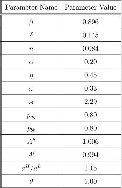
Table 2: Summary of baseline model calibration Parameter Name Parameter Value
0.896
0.145
n 0.084
0.20
0.45
! 0.33
{ 2.29
pgg 0.80
pbb 0.80
Ah 1.006
Al 0.994
aH=aL 1.15
5.2
Model evaluation
Having chosen parameter values to match the …rst moments of the model to those in the
data and to match the volatility of real GDP, in this section we evaluate the model by analysing how key moments of the model compare to those in the data. All variables have
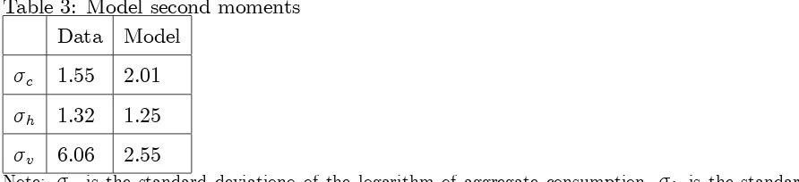
been detrended using the HP …lter (for more details see Appendix G) Table 3 below compares the second moments of the model relative to the data6. The numbers we focus on is the
[image:26.612.88.534.258.360.2]standard deviation of annual aggregate non-durable consumption, aggregate labour hours and the stock market
Table 3: Model second moments Data Model
c 1.55 2.01 h 1.32 1.25 v 6.06 2.55
Note: c is the standard deviationo of the logarithm of aggregate consumption, h is the standard
deviation of the logarithm of aggregate labour hours, v is the standard deviation of the logarithm of stock
prices
The standard deviation of aggregate labour hours in the model are broadly in line with those in the data. The model does less well in the other two key dimensions we use in our
evaluation. Aggregate consumption is too volatile relative to the data. This is a feature of the model that can be improved upon in future work by adding a better means of aggregate
saving. Capital is …xed and the only means of aggregate saving for agents in the model is to purchase intermediate inputs. In addition, due to the low risk free interest rate, workers do
not save and their consumption is as volatile as labour income. In future work I intend to extend the model by adding capital which does not depreciate fully and which can, therefore,
be accumulated in the aggregate, allowing households to smooth consumption better. The volatility of the real value of the S&P 500 in the data is also considerably higher than the
volatility of asset prices in the model.
5.3
Borrowing Constraints and Steady State Productive E¢ciency
In this subsection we consider what would happen in the steady state (i.e. in the absence of aggregate shocks) if the government chooses to impose tighter capital requirements (a lower
value ofe). Perhaps the biggest welfare cost of tighter borrowing constraints arises because borrowing constraints reduce the e¢ciency of the economy. This happens for two reasons.
Firstly, the downpayment requirements on capital acts as a tax on the capital purchases of high productivity entrepreneurs and distorts their production mix relative to the …rst best.
Secondly, borrowing constraints increase the share of low productivity …rms in economic activity, reducing aggregate TFP. Below we explain both of these sources of ine¢ciency.
5.3.1 Capital requirements and the ‘downpayment tax’ on high productivity entrepreneurs
In Appendix H we show that we can write the steady state user cost of capital for high
pro-ductivity entrepreneurs in the tax wedge form popularised by Chari, Kehoe and McGrattan (2007):
uHt = qt
" et
Rt + 1 et
RH t+1
#
qt+1
= uLt 1 + t e
where the tax is given by the following expression
t et = 1 et qt uL
t
1 1 Rt RH
t+1
(20)
The collateral requirement acts like a tax on the capital purchases of constrained pro-ducers. The size of the tax is determined by the followign factors. First of all, the tax is
increasing in the required downpayment on capital goods 1 et. This fraction determines
how much of the capital purchase needs to be …nanced by expensive own savings as opposed
to cheap external funds. The di¤erence between the valuation of internal funds and the market price of loans is given by the 1 Rt
RH
t+1 term in (20). It arises when the borrowing
the collateral constraint forces them to save, this acts to increase their user cost relative to unconstrained low productivity agents. Secondly, the tax is increasing in the price to
rent ratio of capital. This is because a high price to rent ratio increases the internal funds required by a constrained borrower (who needs to have a fraction of the cost of capital as
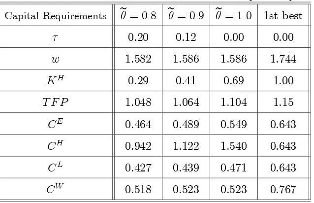
downpayment) relative to an unconstrained borrower (who e¤ectively faces only the user cost). The …rst row in Table 4 below shows how the ‘downpayment tax’ varies with the
value of downpayment requirement. As et - the collateralisability of capital - declines from 1:0and 0:8, the ‘tax’ increases from0 to20%.
Interestingly the impact of capital requirements on the real wage is very small due to two opposing e¤ects. Lower et allows high productivity entrepreneurs to expand production
which boosts TFP and increases wages. But there is another e¤ect. Lower et increases the
user cost of capital and skews the input mix by high productivity entrepreneurs towards
intermediate inputs and labour. The higher labour demand increases the wage. At high levels of et, the share of production done by the e¢cient producers is high and the two
e¤ects o¤set each other leaving the real wage broadly unchanged..
As the last four rows of Table 4 show, the decline in the economy’s e¢ciency due to
higher capital requirements leads to a fall in the steady state consumption of all groups in society. Most strongly a¤ected are high productivity entrepreneurs; their consumption (CH)
declines by more than 30% asefalls towards 0:8from the baseline of 1:0. But other agents in the economy are negatively a¤ected too. Low productivity entrepreneurs’ consumption
(CL) falls 10% largely as a result of the lower wealth of these consumers who accumulate less
wealth during previous productive spells due to the e¤ect of capital requirements. Workers’
Table 4: Selected …rst moments under di¤erent capital requirements
Capital Requirements e= 0:8 e= 0:9 e= 1:0 1st best 0.20 0.12 0.00 0.00
w 1.582 1.586 1.586 1.744
KH 0.29 0.41 0.69 1.00
T F P 1.048 1.064 1.104 1.15
CE 0.464 0.489 0.549 0.643 CH 0.942 1.122 1.540 0.643 CL 0.427 0.439 0.471 0.643 CW 0.518 0.523 0.523 0.767
Notes: is the ’downpayment tax’ rate,wis the wage rate,KH is the share of the capital stock held by high productivity entrepreneurs,T F P is aggregate total factor productivity,CE is average entrepreneurs’
consumption,CH is average high productivity entrepreneurs consumption,CL is average low productivity entrepreneurs consumption,CW is average workers’ consumption.
5.3.2 Capital requirements and the level of TFP
The aggregate level of TFP in this economy is given by the ratio of aggregate output in the economy to the inputs that are used in production.
T F Pt=Ata
H(K) XH HH 1 + (1 K) XL HL 1 (XH +XL) (HH +HL)1
In Appendix I we show that aggregate TFP in the economy is given by the following
expres-sion:
T F Pt=
1 +Kt aH(1 + ( ))1 1 1 + ( )Kt
The downpayment tax and the existence of ine¢cient production under binding borrow-ing constraints endogenously reduces the economy’s level of TFP. This can be seen in the
last row of Table 5 above. Asedeclines from unity to 0:8, the share of capital held by high producitivity entrepreneurs declines from0:69to0:30, bringing about a decline in aggregate
borrowing constraints bind tightly, not enough funds get into the hands of the high produc-tivity …rms. As a result, the economy operates within the production possibility frontier
because some of the scarce capital input is held by low productivity …rms.
5.4
Borrowing Constraints and Aggregate Volatility in the
Sto-chastic Economy
In this subsection we consider how the imposition of capital requirements a¤ect the equilib-rium of the economy with aggregate uncertainty. Here we focus on the ways in which capital
requirements a¤ect the volatility of aggregate consumption as well as the consumption of di¤erent groups and link it to the endogenous ‡uctuations in TFP which arise due to the
ampli…cation mechanism.
Leverage leads to a reallocation of capital between high and low productivity
entrepre-neurs over the business cycle. This happens through the standard collateral ampli…cation mechanism of Kiyotaki and Moore (1997), which can cause substantial endogenous
‡uctu-ations in TFP amplifying the normal shocks to technology over the business cycle. The mechansim which generates this ampli…cation is the following. When the aggregate
produc-tivity state At changes (say, it falls), this reduces the capital price in both the borrowing constrained and in the ‘…rst best’ economy. But whereas in the ‘…rst best’ world, there is
very little additional propagation, in the credit constrained (leverage …nanced) economy, the fall in asset prices impacts the wealth of high productivity and low productivity agents
dif-ferently. Because they are leveraged, high productivity entrepreneurs are badly a¤ected and have to scale down their capital investments because they can no longer a¤ord the required
downpayment as well as the cost of the capital input needed to operate productive projects with a large capital input. The purchasers of capital are the low productivity entrepreneurs
and consequently the economy’s aggregate TFP declines as ine¢cient production expands. The additional fall in TFP puts further downward pressure on capital prices and on the
wealth and borrowing capacity of high productivity entrepreneurs. This is the ampli…cation channel of Kiyotaki and Moore (1997): small declines in the economy’s aggregate technology
the original technology shock. The ampli…cation mechanism is very important because its quantitative strength will be a crucial determinant of whether capital requirements can be
[image:31.612.88.434.141.280.2]welfare improving or not.
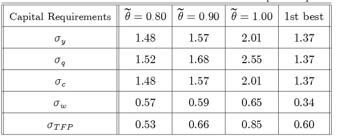
Table 5: Selected second moments under di¤erent capital requirements
Capital Requirements e= 0:80 e= 0:90 e= 1:00 1st best
y 1.48 1.57 2.01 1.37
q 1.52 1.68 2.55 1.37
c 1.48 1.57 2.01 1.37
w 0.57 0.59 0.65 0.34
T F P 0.53 0.66 0.85 0.60
Note: y is the standard deviation of the log of output, q is the standard deviation of the log of
the capital price, c is the standard deviation of the log of aggregate consumption, T F P is the standard
deviation of the log of aggregate total factor productivity, w is the standard deviation of the log of
the real wage rate.
Cordoba and Ripoll (2004) have argued that the amount of ampli…cation in the Kiyotaki
and Moore (1997) framework is very small when one assumes concave utility and decreasing returns to scale in production. They show that large ampli…cation needs a large
produc-tivity gap, a large share of constrained agents in production and substantial reallocation of collateral in response to shocks. Cordoba and Ripoll (2004) …nd that, in particular, there
is a trade o¤ between having a large productivity gap and having a lot of production in the hands of constrained entrepreneurs. This is because they assume decreasing returns to
scale at the plant level. When constrained …rms are very small and their output is low they are much more productive than the larger unconstrained …rms. But the downside is that
their share in total output is low. At the other extreme, when constrained …rms are large, their productivity advantage relative to unconstrained ones is small. In both cases, at least
one condition for large ampli…cation is not satis…ed and so the additional volatility from the model is negligible.
output are, respectively, 38% and 45% higher compared to the …rst best while the standard deviation of the capital price is 84% higher. So contrary to the results in Cordoba and
Ripoll (2004) we get quantitatively large ampli…cation from the framework. Our di¤erences from Cordoba and Ripoll (2004) arise from one main source - our assumption of constant
returns to scale to all factors at the plant level. Even though we have decreasing returns to the collateral factor (capital), the production function is constant returns in all the three
factors. This means that in our calibration we do not face the trade o¤ between the size of the productivity gap and the share of constrained producers in economic activity. The
productivity gap is largely driven by the value ofaH as well as the ‘downpayment tax’ ( ).
It is independent of the level of output at any individual …rm. When we add the e¤ects of
leverage (again realistically calibrated to match US data), we get substantial re-allocation of collateral between high and low productivity entrepreneurs as asset prices ‡uctuate. So
Cordoba and Ripoll’s conditions for ampli…cation are satis…ed and this explains why our constrained economy is so much more volatile relative to the ‘…rst best’. Our results are
similar to those in Vlieghe (2005) who found something very similar in a version of Kiyotaki (1998) with nominal rigidities. In his model (which also featured constant returns to all
fac-tors) ampli…cation was very substantial showing the potential of the framework to propagate shocks.
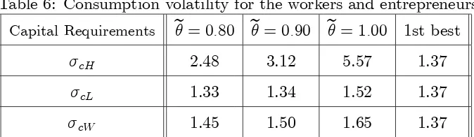
In addition to the ampli…cation of aggregate ‡uctuations, leverage concentrates the ag-gregate risk in the hands of only a small subset of agents in the economy. When capital
is largely held by high productivity entrepreneurs who …nance their capital holdings using simple debt, risk sharing between the two groups deteriorates. We can see this in Table
6 below which shows the variance of the aggregate consumption of the two groups. This di¤erence grows as credit constraints are relaxed due to the increasing collateralisability of
Table 6: Consumption volatility for the workers and entrepreneurs7
Capital Requirements e= 0:80 e= 0:90 e= 1:00 1st best
cH 2.48 3.12 5.57 1.37
cL 1.33 1.34 1.52 1.37
cW 1.45 1.50 1.65 1.37
Note: cH is the unconditional standard deviation of the log of the consumption of high productivity
entrepreneurs, cLis the unconditional standard deviation of the log of the consumption of low productivity
entrepreneurs, cL is the unconditional standard deviation of the log of the consumption of workers.
This result is not surprising. The low productivity entrepreneurs hold largely riskless
debt and small positions in risky capital. In contrast, high productivity entrepreneurs hold leveraged positions in risky capital. This asymmetry in the asset holdings of the two groups
leads to a concentration of the aggregate risk in the economy into the hands of very few (high productivity) individuals whose consumption ‡uctuates very substantially. Our results are
in line with the …ndings of Vissing-Jorgensen and Parker (2009) who …nd that the aggregate risk is borne by a small fraction of high consumption/high income households. Tightening
…rms’ access to borrowing reduces this asymmetry in the riskiness of di¤erent indivdiuals’ portfolios and consequently reduces the volatility in their relative consumption levels over
the business cycle.8
5.5
Discussion
In this section we examined the quantitative signi…cance of four ways in which the credit
constrained economy is distorted relative to the …rst best. These distortions, however, do
7Note that these consumption volatilities refer to the standard deviation of the consumption of all agents
who happen to be high or low productivity at a given point in time. They are not the expected standard
deviation of the consumption of the people who are high or low productivity at time0 when the policy is
decided upon.
Nevertheless we think these numbers are informative of the kind of consumption volatility caused by
aggregate uncertainty. It illustrates the fact that high productivity entrepreneurs face a lot of risks to their
net worth because of leverage and this causes their consumption to be much more volatile ex post.
8In the limit, when no borrowing is allowed and all production is entirely net worth …nanced, both types
not necessarily imply that the economy is constrained ine¢cient. As long as the government cannot do anything directly about borrowing constraints, many of these distortions will be
an unavoidable consequence of credit market imperfections.
For example, any deviations of the economy’s steady state from …rst best would be
constrained e¢cient. The trade o¤ between productive e¢ciency and consumption smoothing is identical for private individuals and for the government. Private borrowers with good
productive opportunities choose to borrow up to the limit and experience a steeply sloped consumption path because the rates of return they can earn on productive projects are
much better compared to the cost of debt. The government will make an identical decision because it can redistribute capital holdings between the two groups and compensate the low
productivity …rms for their lost output while still making the high productivity borrowers better o¤. The only constraint on this redistribution is the collateral constraint, which binds
for the government in the same way as it binds for the laissez faire economy.
In a stochastic environment, the e¢ciency properties of the competitive equilibrium
change. The collateral ampli…cation mechanism of Kiyotaki and Moore (1997) introduces feedback e¤ects between asset prices, the net worth of leveraged borrowers and the tightness
of borrowing constraints. When aggregate productivity switches from high to low, asset prices fall and this has a disproportionately negative e¤ect on the net worth of leveraged
high productivity borrowers. Because part of the capital purchase and the whole of the intermediate input purchase is non-collateralisable, borrowers need their own net worth in
order to produce on a large scale. Therefore the fall in the net worth of high productivity borrowers reduces the amount of capital they can invest in production and forces them to
scale down their capital holdings. The low productivity agents absorb the capital sold by the high productivity ones but only at lower prices. But this fall in the price of capital further
damages the net worth of leveraged …rms and forces them to cut their capital holdings even further. This completes the ‘credit cycle’, amplifying and propagating small shocks into
larger ‡uctuations in output, TFP and asset prices.
Where does the ine¢ciency of private leverage come from? As identi…ed in Lorenzoni
the allocative e¢ciency of the economy. The forced sales of leveraged borrowers depress asset prices and tighten the credit constraints of all other constrained borrowers, forcing them to
sell assets themselves9.
6
The Model Economy under Capital Requirements
In this section we turn to the main question of this research: are private leverage decisions
optimal from a social point of view? From the work of Lorenzoni (2008) and Korinek (2009) we know that, qualitatively, the answer is ‘no’. Here we examine whether, quantitatively,
the ine¢ciency is large or small.
We assume that capital requirements are chosen by a benevolent government who
max-imises a social welfare function which weights the values of all agents in the economy. The government is subject to the same collateral and budget constraints facing private agents. So
any di¤erences in private and social leverage choices are due to the market price externality
discussed above.
6.1
The Government’s Problem
The government optimises the coe¢cient on a simple state contingent capital requirement
rule
et= min exp i0+ i1lndt+ i2lnZt ; (21) in order to maximise the following social welfare function
0 = max
f ig E0
" X
i &iE
1
X
t=0 t
lncit
#
+&W
1
X
t=0 t
ln CtW {
(Ht)1+! 1 +!
!
(22)
9But although such pecuniary externalities exist they are not always quantitatively signi…cant. For
example, Guerrieri (2007) examines the constrained e¢ciency of a competitive labour market search model
with private information and limited commitment. In her model, workers take the value of the outside
unemployment option as given while the planner recognises that it is endogenous because the expected
value of job matches a¤ects the continuation value of the unemployed. Although Guerrieri (2007) identi…es
this very interesting source of ine¢ciency of the competitive equilibrium, she …nds that, quantitatively, the
where &i
E is the Pareto-Negishi weight on entrepreneur i while &W is the Pareto-Negishi
weight on the workers. We do not consider any other policy instruments.10 Note that the
capital requirements et is constrained by the exogenously given limit .
et 6
In other words the government has no advantage in enforcing debt repayment over the
private sector and therefore it cannot choose looser capital requirements than the market. The policy rule (21) allows the capital requirement to undergo mean shifts as the aggregate
productivity state changes. Capital requirements also can respond to changes in the other aggregate state variables - total wealthwtand the share of wealth held by high productivity
people dt. Once the government has chosen capital requirements, the collateral constraint in the regulated economy becomes:
bt6 etEtqt+1kt (23)
Private agents then perform exactly the same maximisation problem as in the unregulated
economy, but the collateral constraint they now face may be tighter if et < in some states
of the world.
In Appendix C we show that the value function of the two types of entrepreneurs at time
0 depends on the net present value of future expected log rates of return on wealth as well
10We do not solve a social planning problem because the collateral constraints in our economy depend on
prices and these do not admit to a simple closed form solution in the same way as in Lorenzoni (2008) and
Korinek (2009).
In future work, we intend to solve for the full Ramsay problem. We do not do this here because it
complicates the solution of the model. At the same time the policy we consider does capture a lot of
intuitive features about the way capital requirement policy may be implemented. It is fully state contingent
and it is conducted under commitment because the government chooses the i
coe¢cients at the beginning
of time and sticks to them for ever.
Our policy rule is, therefore, similar to the ‘Optimal non-inertial plan’ popularised by Woodford (2003)
because it is conducted under commitment (the central bank opimises its coe¢cients in a once and for all
fashion) but without responding to lagged variables (which is what the optimal Ramsay commitment policy
as the logarithm of current …nancial wealth.
Vi(X0) = 'i(X0) + lnz0
1 ; i=H; L
where 'i(X0) is the net present value of future rates of return on wealth and z0 is time 0
…nancial wealth.
'i(Xt) = ln (1 ) + ln
1 + maxxt;kt;ht;bt
Et
"
ln Ri t+1
1 +'
i(Xt+1)
#
We assume a particular initial wealth distribution in which all high and all low productivity entrepreneurs have an initial level of wealth equal to the group average in the ‘no regulation’
steady state. This allows us to consider the following social welfare function which weights the utilities of the three groups by the inverse of their marginal utility of consumption
evaluated at the initial wealth distribution (more details in Appendix K):
0 = max
f ig E0 &
H 'H(X 0) +
lnZH 0 1 +&
L 'L(X 0) +
lnZL 0 1 +&
WVW(X
0) (24)
where 'H(X0) and 'L(X0) are the NPVs of future expected log rates of return on wealth
for the two groups of entrepreneurs whileZH
0 andZ0L are the initial wealth levels of the high
and low productivity entrepreneurs.
6.2
When is private leverage excessive?
The benevolent government chooses and commits to a time invariant capital requirement
function etwhich maximises social welfare (24). The government cares about three things in
(24). It wants to maximise the Pareto weighted average of the net present expected value of
log returns on wealth for the two types of entrepreneurs. These are the the'H
0 and 'L0 terms
in the social welfare function. But it also wants to maximise the welfare of workers which
depends on the average level and volatility of real wages. Finally, the government cares about the current …nancial wealth of entrepreneurs too. It knows that any policy announcement
will immediately be re‡ected in the capital price, impacting on the wealth of the two groups and it takes this into account when designing the optimal policy. In the next section we will