Munich Personal RePEc Archive
Argentina-Canada from 1870: Explaining
the dynamics of divergence
González, Germán and Viego, Valentina
CONICET - Departamento de Economía, Universidad Nacional del
Sur, Departamento de Economía, Universidad Nacional del Sur
June 2009
Online at
https://mpra.ub.uni-muenchen.de/18394/
Argentina-Canada from 1870: Explaining the dynamics of divergence
Germán H. González
CONICET y UNS
V alentina Viego
UNS
Work in progress
This version: June 2009
COMMENTS ARE WELCOME
Departamento de Economía, Universidad Nacional del Sur.
12 de Octubre 1198, 7mo piso. D8000CTX Bahía Blanca, Argentina
Tel. fax. +54 291 4595138 (interno 2735)
Abstract
Argentina and Canada started their industrialization processes while exporting natural
resources and importing capital goods. These two nations were sparsely populated but received
significant inflows of European immigrants since the second half of the nineteenth century.
Until the start of World War II, both economies experienced similar per-capita GDPs.
However, the gap between both per-capita GDPs began to grow, widening throughout the
between both economies. We confirm that while Canada was drawn into a successful path due
to the adjacency with a bigger and complementary economy, Argentina fell into a “staple trap”.
Keywords: Relative per-capita GDPs, development accounting, total factor productivity,
Argentina, Canada
JEL: N12 – N16 – O11 – O57
Resumen
Argentina y Canadá comenzaron sus procesos de industrialización al tiempo que exportaban
recursos naturales e importaban bienes de capital. Ambas se encontraban escasas de población
y recibieron un significativo flujo de inmigrantes europeos a comienzos de la segunda mitad
del siglo XIX. A comienzos de la Segunda Guerra Mundial, ambas economías poseían
similares PBI per capita. Sin embargo, la brecha en el ingreso comenzó a ampliarse,
profundizándose a lo largo del siglo. El trabajo ofrece un estudio empírico de los determinantes
profundos del proceso de divergencia entre ambas economías, y confirma que, mientras Canadá
siguió un sendero exitoso debido a la adyacencia con una economía complementaria y de
mayor tamaño, Argentina entro en una staple trap.
Palabras claves: PIB per capita relativo, contabilidad del desarrollo, productividad total de los
factores, Argentina, Canadá
Argentina-Canada from 1870: Explaining the dynamics of divergence
1. Introduction
Argentina and Canada showed until the beginning of World War II (WWII) similar per-capita
GDPs. Both economies started their industrialization processes by exporting natural resources
and importing capital goods. Both were sparsely populated, but received significant inflows of
1930s, however the gap between both per-capita GDPs began to grow, accelerating later in the
century. This experience was examined by a literature that, on the one hand, tries to determine
the precise moment in which the divergence began. On the other hand, it tries to explain why
Argentina could not break that trend and catch up with Canada.
The divergence between both countries during last century seems to be particularly relevant for
Argentina for, at least, three reasons. First, at the same time that Canada reached a level of
per-capita GDP corresponding to an advanced economy, Argentina lost its momentum.
Understanding why this happened may help to overcome this handicap. Second, Canada has
been seen as a benchmark for Argentina because of the widespread idea in the historiography
that Argentina could have followed a similar path. Third, interesting questions about economic
policy arise from this comparison. For example, are exogenous or endogenous the factors
which lead to the dismal performance of Argentina? It would be worth to examine the
differences among policies of international trade in both countries. Should Argentina redefine
its development process acting directly over the apparent causes of the increasing divergence
with Canada or should exploit more subtle causes of this phenomenon?
This paper has two aims. First, it shows that any explanation of the diverging path between
Canada and Argentina must consider the peculiar Canadian proximity to United States. Second,
the Staple theory is a useful theoretical framework to do that. While Canada was drawn into a
successful path due to the adjacency with a bigger and complementary economy, Argentina fell
into a “staple trap”. In evidencing our affirmations, we carry out an empirical study of the deep
determinants (Rodrik, 2003) of the divergence process between both economies. Although
similar studies have been run, our study uses a different methodology. More specifically, we
run econometric tests of some old and new hypotheses, while specific points in time we used to
To do that, we first follow the works of King and Levine (1994), Klenow and Rodriguez-Clare
(1997) and Hall and Jones (1999), and offer a development accounting framework. This
exercise does not directly address why output per capita differs across countries nor why the
gap increased, but it provides estimates of total factor productivity, GDP shares of production
factors, and an approximation of the contributions of physical and human capital, and
technological progress to differences in levels of income per capita. We then use the results to
explain across country income differentials in levels regressingthe deficit in the Argentine
performance on geography, integration and social infrastructure.
The paper contains six sections. In the second section we shall establish the absence of
convergence and catching-up of Argentina. The third section presents the fundamental issues
highlighted by the literature on Canadian and Argentine economic development. According to
Temple (1999), historians can usefully point to particular factors that others are likely to miss.
The statistical and econometric work, perhaps using cross-sections variation, is often necessary
to quantify the importance of the potentially relevant factors. In this sense, the forth section
introduces the methodology and the fifth presents the empirical results. Final considerations are
discussed in the sixth section.
2. Argentina’s catch-up dynamics
From the 1870s to the 1930s Argentina shows an extraordinary dynamic macroeconomic
performance with an income, income per capita and GDP growth comparable to current
developed countries. Between 1900 and 1930 Argentina per capita GDP did not show notable
differences with per capita GDP of Austria, Germany, France and Sweden. Its performance was
and Taylor “Argentina’s 1913 income level was clearly in the world top ten, and almost the top
five. Whatever its exact status in 1913, for all practical purposes Argentina was an advanced
country” (2003: 3). As result, Argentina received substantial foreign direct investment and
massive labor immigration from Europe. Although the per-capita GDPs of US, Australia and
New Zealand were always over the Canadian and Argentine ones, all these countries seemed to
be in the same convergence club.
Up to the 1930s the picture changed. Moreover the data of Argentine’s economic performance
since the end of the WWII shows that the country initiated a diverging path compared to the
evolution of the set of economies with similar origin and others. Argentina’s ratio to OECD
income fell from 80 percent in 1913 to 65 percent in 1973, and a mere 43 percent in 1987 (della
Paolera and Taylor, 2003). Miguez (2005: 483) point out that between 1913 and 1989
Argentina grew to 0.74% annual while the world-wide economy did it to 2%.
In order to compare different paths of development between Canada and Argentina, we analyze
data on per capita GDP of both countries relative to the US. More specifically, we study the
behavior of the performance of Canada and Argentina with respect to the performance of the
US over time:
= Per capita GDP of Country i in year t
u
it US per capita GDP in year t
where the role of country i is occupied for Canada and Argentina, and the US is taken as the
benchmark.
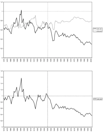
Figure 1. (a) Performance of Argentina and Canada relative to United States, and (b) Argentine
0 0,2 0,4 0,6 0,8 1 1,2 1 8 70 1 8 75 1 8 80 1 8 85 1 8 90 1 8 95 1 9 00 1 9 05 1 9 10 1 9 15 1 9 20 1 9 25 1 9 30 1 9 35 1 9 40 1 9 45 1 9 50 1 9 55 1 9 60 1 9 65 1 9 70 1 9 75 1 9 80 1 9 85 1 9 90 1 9 95 2 0 00 u(ar,us) u(ca,us) 0 0,2 0,4 0,6 0,8 1 1,2 1,4 1,6 1,8 1 8 70 1 8 75 1 8 80 1 8 85 1 8 90 1 8 95 1 9 00 1 9 05 1 9 10 1 9 15 1 9 20 1 9 25 1 9 30 1 9 35 1 9 40 1 9 45 1 9 50 1 9 55 1 9 60 1 9 65 1 9 70 1 9 75 1 9 80 1 9 85 1 9 90 1 9 95 2 0 00 u(ar,ca)
Sources: Maddison (2006) and Ferreres (2005)
Figure 1(a) plots the evolution of uit for a long period of years. Several interesting facts emerge.
First, the existence of at least two large dissimilar periods: one lasting from the end of XIXth
century to the mid-1930s, the other starting in the mid-1930s lasting until the present day. The
first is characterized by a similar path of relative performance,the other shows Canada
[image:7.595.124.481.66.535.2]Canada’s relative per capita GDP seems to show an inverse association between the mid-1900s
and mid-1930s.
Finally, Argentina’s per-capita GDP steadily decreases between the end of WWII and the 1973
Oil Crisis, while Canada almost reaches its historical maximum at the end of this period. The
first observation shows when Argentina lost its momentum. Argentina experienced the last
peak in their per capita income relative to US before mid-1930s. The second one invites us to
deepen the analysis because this period reveals the basis of the subsequent divergence
behavior1. The dismal performance between the two economies after mid-1930s became
apparent in the figure 1(b) where Canada is taken as benchmark.
In the next section we discuss the historiography regarding the Argentine collapse during
twentieth century. In light of this literature review we reduce the principal approaches to simple
abstract relationships that we test econometrically. In this manner, we reduce the range of
possible explanations.
3. Some previous studies
3.1. Studies on Canadian economic development
It is impossible to begin a survey of the studies on Canadian economic development without
mentioning the staples theory of Mackintosh and Innis. Classic essays2 about this approach are
Buckley (1958), Aitken (1958), North (1955; 1956; 1959), Baldwin (1956), Bertram (1963),
and the discussion initiated by Chambers and Gordon (1966, 1967) and followed by Dales et al.
(1967), Bertram (1973), and Grant (1974) among others.
1 This hypothesis is also presented by Korol (1991) after an interesting review of the comparative studies of
Argentine decline.
“Traditionally, staple production is defined as comprising primary (resource) activities and
those primary manufacturing activities, such as lumber, pulp, and paper mills and fish
processing plants, in which resources are major inputs to the production process” (Hayter and
Barnes, 2000: 158). The country possesses a comparative advantage in a natural resource or
staple industry and this advantage is so great that this exporting sector becomes “the leading
sector of the economy and sets the pace for economic growth” (Watkins, 1963: 144). Economic
development is then a chain of spread effects of the export sector that transform the domestic
economy and society. Watkins wrote that those spread effects are realized through three types
of well-known linkages effects: backward, forward and final demand. Altman adds the fiscal
linkage to the previous list. This last refers to “the income that the state receives as a result of
staple and staple-related production” and “result in the investment in social overhead, such as
transportation, education, research and development. Fiscal linkages can make the staple
economy more efficient and competitive… On the other hand, the state can use its
staple-related stream of income unproductively” (2003: 237).
Watkins also emphasizes two potential impediments to development that stem from staples
production. First, “staple exporters –specifically, those exercising political control- will
develop an inhibiting export mentality, resulting in an overconcentration of resources in the
export sector and a reluctance to promote domestic development” (1963: 150). Second,
“sustained growth requires the capacity to shift attention to new foreign or domestic markets.
The former requires a favorable combination of external demand and available resources. The
latter requires a population base and level of per capita income that permit taking advantage of
the economies of scale in modern industrialism. Both require institutions and values consistent
with transformation and that requires the good fortune of having avoided specialization in the
Once a region specializes in producing staples, it then finds it very difficult to reconfigure
production into other types of sectors. The result is susceptibility to already volatile resource
international prices, making the staples economy especially prone to crisis (Hayter and Barnes,
2000). “If the pitfalls are avoided –if staples generate strong linkage effects which are
adequately exploited- then eventually the economy will grow and diversify to the point where
the appellation staple economy will no longer suffice” (Watkins, 1963: 151)
Currently, there seems to be consensus about some points in time or circumstances that are
empirical milestones in an economic analysis of the post-Confederation Canadian history3: the
National Policy of Tariff (1879), the Import Duties Act (1919) and the Imperial Preference
(1932, Ottawa Conference), and the formal alignment with US after the Reciprocal Trade
Agreements Act (1934).
The National Policy of Tariff consisted in a development policy to stimulate import
substitution industrialization4. But the intent of the government and businessmen was to protect
the Canadian market and reach equilibrium in the balance of payments rather than create
conditions to promote industrialization (Lucchini, 2002). di Tella (2007) said that tariffs were
necessary for the railway to exist and the railway was indispensable for Canada to exist. The
positive and public acceptance compelled the Liberal party to accept this policy despite a
tradition of upholding the reciprocity treaties for years before.
3 The process of the Canadian independence began with the British North America Act or Constitution Act of
1867 which creates a federal system of government between Province of Canada, Nova Scotia and New Brunswich. Subsequently the Balfour Declaration (1926) established that the ex-colonies were autonomous communities united in common loyalty to the Britannic Crown and the Statute of Westminster (1931) established a status of legislative equality between the self-governing dominions of the British Empire and the UK.
4 The first Canadian-US reciprocity treaty was signed in 1854. There is agreement on understanding it as a
Lucchini (2006) argued that the Canadian industrial sector was constituted by poor-integrated
activities, and it was conducted by local businessmen with scarce foreign capital until 1870.
The positive impact of the new economic program took place through a significant
technological renewal. The technological progress is explained by the exploitation of scale
economies, the early expansion of hydroelectricity, and the increasing share of US capital on
domestic firms that took advantage of protected market. The industry concentrated over a
smaller number of firms controlled by foreign capital. Although this early industrial
development, the agricultural sector maintained their leading role. The period between 1901
and 1911 has been characterized by a boom in Canadian wheat exports and considered by
many scholars as having been critical to Canada’s economic development (Altman, 2003).
The Import Duties Act (1919) and the Imperial Preference (1932) lowered duties to the
production with Imperial origin, and products that came from the Commonwealth, respectively.
The industrial businessmen united in the Canadian Manufacturers’ Association –to a large
extent, these men were executives of subsidiary of US firms- proposed an Imperial import
substitution policy similar to the Canadian one. The preferential treatment was given by the
Britannic Crown to a substantial number of Canadian manufactures from 1919. During the
years of the Great Depression, UK hardened its stance as response to the trade police of US and
Continental Europe, and Canada was obliged to make an effort to keep the British market. As
result, the Imperial Preference was agreed upon at the 1932 Ottawa Conference, and Canada
government saw it as “a means of putting pressure on the US to reverse its 1930 tariff
increases” (Pomfret, 2000: 118). However, one of the indirect effects of this policy was the
growth of the US investment in Canada with positive and transcendent implications on
Canada takes away from confrontation with US by the enactment of the Reciprocal Trade
Agreements Act (1934). Later, Canada signs a new bilateral agreement in 1935, an agreement
with US and UK in 1938. After 1947, Canada embraced multilateralism following those
countries, principally US (Pomfret, 2000). 5
3.2. Studies on Argentine economic development
Asencio (1995: 13) assumed that disentangling the Argentine enigma is not lamentably an
original determination. Not only taken Argentina alone, but through the comparison with
Canada, Australia6, United States7 and other countries with, at least notionally, similar initial
characteristics. In the first case, Ferrer (1963), Díaz Alejandro (1970), di Tella and Zymelman
(1967, 1973), Cortés Conde (1997; 1998), Vázquez-Presedo (1992) are classic references
between historians and economists. More recent efforts are della Paolera and Taylor (2003) and
Rapoport (2005).
Between the Argentinists exists a certain agreement on describing the Argentine economic
structure between 1880 and 1930 as an agro-exporting peripheral countries. Similar to Canada,
the economic growth was closely related with the primary sector and the government and
foreign investment in basic infrastructure. Moreover, the shortage of labor force made possible
the coexistence of the enriched elite not necessarily associated with the production and export
of primary goods, and the work class with a relatively high income compared with the income
in the European economies. This last characteristic together with the perspectives of prosperity,
promoted an important wave of immigrants and a substantial flow of foreign investment
attracted by the domestic market in expansion. During that period, the trade policy was
5 Finally, Canada liberalized trade substantially with the implementation of Canada-US Free Trade Agreement in
1989 and subsequently with the North American Free Trade Agreement (NAFTA).
6 See, for instance, Fogarty et al. (1979) and Duncan and Fogarty (1984, especially their annotated bibliography
from page 177 to 199). More recently Gerchunoff and Fajgelbaum (2006) and the set of papers presented in the 2007 Seminary John Fogarty at CEI (Argentina).
essentially free-trade except for some protected sectors (Lucchini, 2002). The Argentine history
did not begin in 1880; however it is a widespread opinion among Argentinists that was that
year when there were consolidated the central government and the institutions needed for an
economic program based in agro-exporting sector.
In analyzing Argentine development, Geller (1975), Cincunegui (1982) and Fogarty (1985)
applied the staple theory. Accordingly to those authors, the model could be used to explain the
early stages of development when the primary sector had such influence –direct and indirect-
over the economy. Afterwards, other sectors replaced it and the model loses its explanatory
power. Fogarty concludes that explanations about poor Argentine development are to be found
in supply-side factors such as “entrepreneurship and capacity for innovation or in
non-economic factors like the institutional environment and government policies” (Korol, 1991).
There is a vast discussion about what are the processes that explain the delay of Argentina
taken into consideration the period of similarity with Canada. Many studies use the
comparative method to analyze the Argentine performance. The Canada-Argentina comparison
has been particularly fruitful8. Generally, the analyses converge on the reaction of the
government and other economic agents to the “historical accidents of relevance”9. They point
out political, institutional and even geographical and sociological constraints to the process of
decision making.
8 Usual references are the collections of papers edited by Platt and G. di Tella (1985, 1986), Taylor (1994),
Solberg (1987), Adelman (1992, 1992b, 1994), Teichman (1982) , Sabato (1988), Waisman (1987). More close in time, Asencio (1995), Chudnovsky et al. (2000), Muchnik (2003), Miguez (2005), Sanz Villarroya (2005), T. Di Tella (2007), and Prados de la Escosura y Sanz Villarroya (2008).
Gerchunoff and Fajgelbaum argued that after the crisis of WWI “in the middle of the
uncertainty, each country10… sought refuge in its recent history to define future policies.
Argentine policymakers had no reason to deny what had produced huge returns, and, as a
consequence, the deep political changes that followed the electoral reform of 1912 were
accompanied by barely superficial changes in economy… it became evident that the bet on
trade stayed firm, and even the inherited protectionism was losing strength something opposite
to what was happening in other latitudes” (2005: 16-17).
After 1929 “there was not much to argue in a world devastated from the commercial and
financial viewpoint,… it was necessary to promote manufacturing, to stimulate the expansion
of the domestic market and to obtain as much profit as was possible… from the battered export
activities” (p. 18-19). These authors argued that the explanation about the different paths until
WWII could be explained by a time lag. Nevertheless, WWII meant not only a new closure of
trade that encouraged import substitution, but an important possibility for allying oneself with a
new world-wide economic power. In contrast, Argentina bet on the external conditions would
be the appropriate for the balance of payments and kept the commercial alliance with UK while
flirted with Axis powers. The terms of trade fell after the war and “the fifties were dominated
by the stop-and-go, and when exports started resurging, Argentina had become the arena of a
distributive struggle” (p. 26). At this point, the geopolitical aspects play an important role in
this story of divergence. Could this analysis made for the comparative development analysis
between Argentina and Australia, be useful for our purposes?
The Canada-Argentina historiography seems to answer affirmatively. Rapoport (1994) argued
that until the XXth century, Argentina’s system of land distribution stamped a particular
production character –principally stockbreeding- and decided the most influential interest
group11. The preponderance of the landowner over the remaining political groups would
explain, according to Rapoport, the strong Anglo-argentine conexion around the middle of
XXth century with lasting effects over the economy, specifically, the excessive relevance of
beef and the delay in the productive diversification.
Rapoport mentioned that after the WWI, US investment growth principally in those sectors
with cost advantages and access to the British market12. Despite the trade between Argentina
and US grew notably during the war, after the peace the US imports with Argentine origin
returned to pre-war level while its exports kept high. The imbalance with US and the stagnation
of the exports towards Europe led Argentine economy to experience difficulty with balance of
payments after the 1930s. Hence, the Imperial preferences became a hazard for the sectors
related with the primary exporters: In that moment 33% of the production was exported toward
UK. Argentina made an effort to keep the market but results were mediocre. In 1933 both
countries signed the Roca-Runciman Agreement; the pact was only useful for reducing the
backward movement of this market but not to alter its existence (Asencio, 1995) meanwhile
Argentina gradually moved away from US economy13. The Great Depression led Argentina to
seek refuge in the domestic market; however it did not get the expected results14.
11 Asencio (1995) argued that the agrarian revolution was not possible until the massive immigration because
cultural, technological and economic factors and the combination promoted a process of collateral expansion of the agriculture dependent on the stockbreeding expansion. Between the factors of delay the author mentions the generalized view of the farming activities as non-noble, the limited propensity for scientific advances and the lack of means of transport and storage. But the massive immigration also had a delay due to some factors, one of them the access to land. Neither the early Rivadavia’s attempt (1922) nor the Liberal policies of Mitre, Sarmiento and the Avellaneda Law (1876) had the effects of the Canadian Homestead Act (1872). Between 1833 and 1853, and even some years after of the Roca’s Big Campaign of Desert (1879), the distribution of land followed a prize-giving pattern with a tendency to the concentration of land into large establishments.
12 Towards the 1920s, US capital took control of the meat processing industry (Smith, 1983).
13 The temporary improvement during the beginning of WWII was lost because the Argentine neutrality.
14 In terms of Ferrer (1963) there was an error of design of economic policy; it had as consequence a
In contrast, despite the institutional links with UK, at the beginning of the XXth century
Canada was an economy with a diversified production and less dependence on primary exports.
Moreover, the division of land into smallholdings and the early industrialization process made
that the more powerful interest group was the manufacturer one (Lucchini, 2006) and its
principal objective to hold the economic links with US without losing the advantage of being a
member of the Commonwealth15. Despite the toughening of the US policy and the Ottawa
response reduce outstandingly the trade between both countries, the treaty of reciprocal
preferences enacted in 1935 returned to the beginning the commercial plane while the
alignment with US to the WWII reinforced the political relationship so that economic links
were strong like never before.
4. Methodology
4.1. Development accounting
In Caselli (2005: 681) we find a synopsis of what we know as development accounting: it “uses
cross-country data on output and inputs, at one point in time, to assess the relative contribution
of differences in factor quantities, and differences in the efficiency with which those factors are
used, to these vast differences in per-worker incomes”. Similarly, King and Levine (1994)
present Denison’s definition in such terms: “While a development accounting question is what
part of cross-country differences in income per capita is accounted for by differences in
physical capital per capita, a growth accounting question is what part of cross-country
differences in growth rates of output is accounted for by differences in growth rates of capital
per capita”. We consider, agreeing with Hall and Jones (1997), that growth research has not
15 Promfret (2000) mentioned that “At Confederation in 1867 Britain supplied 60 per cent and the USA 32 per cent
provided effective explanations for the extreme diversity in output per worker across countries,
and a study of levels in economic activity could give complementary insights.
Country performance is driven by other fundamental determinants not directly captured in
typical accounting (factor accumulation and technological efficiency). Hall and Jones
highlighted the social infrastructure, defined as the collection of laws, institutions, and
government policies that make up the economic environment, and they considered that “a
perverse infrastructure discourages production in ways that are detrimental to economic
performance” (op. cit.: 174). Their works conclude that when social infrastructure favors
diversion of resources over production, investment in physical capital, skills, and the transfer of
research and technology are reduced. Hence, social infrastructure affects income levels per
worker through each element of the production function.
The concept of social infrastructure is associated with the notion of cultural differences,
presented by Acemoglu (2007). He argues that cultural differences determine individual values,
preferences and beliefs. We could expect that these cultural differences then led to dissimilar
institutional arrangement.
Other sources of direct differences, according to Rodrik (2003), are geography (climate and
resources) and integration to the world economy. Using an expression of Acemoglu,
“geographic differences that affect the environment in which individuals live and that influence
the productivity of agriculture, the availability of natural resources, certain constraints on
individual behavior, or even individual attitudes” (2007: 23). Rodrik argued that geography
also affects income via integration –for example, access to the market and transport costs- and
institutions -e.g. geopolitical considerations and effects of natural resources-booms in quality
All of them argued that this deep or fundamental determinants change slowly or hardly at all in
time. As they, we are interested in the long-run determinants of economic success and not in
the transition dynamics; hence we put special attention to historical episodes that represent an
institutional break or abrupt changes in rules-of-game. In this sense, Rodrik argued that
“moderate changes in country-specific circumstances, often interacting with the external
environment, can produce discontinuous changes in economic performances”.
Our departure point is the development accounting exercises performed by Mankiw, Romer
and Weil (1992), Klenow and Rodriguez-Claire (1997) and Hall and Jones (1999).
Accordingly, consider the following aggregate production function with constant returns,
( )
1Y =K Hα β AL − −α β
where Y represents output, K the (total) stock of physical capital, A is a productivity index, and
L is the number of (employed) workers in the economy. The total stock of human capital is the
product of the average level of human capital, h, and the number of workers (H = ×h L).This
production function can be rearranged as
1 1
Y K H
A
L Y Y
α β
α β α β
− − − −
=
In order to consider per capita income instead of per worker income, let P be total population.
Using the relationship16
Y L Y
P = ×P L,
we rewrite the production function as
16 Blyde and Fernández-Arias (2005) and Manuelli (2005) used similar expression while Hopenhayn and
(1) y l K
( ) ( )
1 H 1 Aα β
α β α β
− − − −
= % %
where y (≡Y P) is per capita income and l (≡L P) is the employment rate; K%(≡K Y) and
H% (≡H Y ) express physical and human capital intensities17. The effect combined of the three
components can be interpreted as the effect of factor accumulation. We follow King and
Levine (1994) and use the Perpetual Inventory Method with steady-state estimates of initial
capital in the construction of K series18. Similarly, we follow Mankiw et al. (1992) to compute
the human capital intensity
H
st
I Y H
n g δ
=
+ +
%
where IH is the inversion in human capital, gst is the steady-state growth rate of the country, n
is the growth rate of the country’s population, and δ is the rate at which human capital
depreciate19. IH/Y is computed using
15 19 population secondary school enrolment rate
15 64 population
H
I Y
−
= ×
−
which approximates the percentage of the working-age population that is in secondary school.
The last component in (1), the productivity index or total factor productivity, partially reflects
the level of technology. However, this variable also could capture unemployment of available
resources and technological inefficiency. Whereas resource unemployment could be considered
17 We use the decomposition in terms of capital intensity rather than the capital per worker ratio due to the reasons
mentioned in Hall and Jones (1999). Mainly, we could distinguish between an increase in output that is fundamentally due to the increase in productivity and the increase in output that is due to factor accumulation. Authors that use the same decomposition approach are Mankiw, Romer and Weil (1992), Klenow and Rodriguez (1997) and Hopenhayn and Neumeyer (2004).
18 For initial GDP we took the average of the period 1910-13 while for the inversion rate in the steady state we
took the average for the period 1915-84. 19 The same values of g
st, n and δ are used for both K and H estimations. The rate gst is computed following
Easterly et al. (1993) and King and Levine (1994): gst =λg+ −(1 λ)gw; where g is the average of the annual
GDP growth rate for the country, gW is the world-wide average growth rate and λ = 0.25. Parameter n is the
as an important measurement error in some studies, it is relatively unimportant for us. Mainly,
with Blyde and Fernández-Arias, we are particularly interested in the explanation of long-run
gaps between countries instead of cyclical variations in the utilization of the production factors.
Then, it is possible to undertake development accounting on the basis of the production
function above. That is, we can take the ratio of two national measures of per capita income
using expression (1),
(2) i i i 1 i 1 i
j j j j j
y l K H A
y l K H A
α β
α β α β
− − − − = % % % % .
Given data on relative quantities of factor production and specific values of α and β, we can
measure cross-country differences in TFP , relationship expressed here as Ai/Aj, as residuals:
(3)
1 1
i j i
j
i j i j i j
y y A
A
l l K K H H
α β
α β α β
− − − − = % % % % .
To describe the extent to which labor, physical and human capital and TFP account for
cross-country differences in per capita income, we begin by constructing the following ratios
(4) ln
ln i j li i j l l y y
ϕ =
(
)
(1 )ln ln i j Ki i j K K y y
α α β
ϕ − − = % %
(
)
(1 )ln ln i j Hi i j H H y y
β α β
ϕ − − = % % ln ln i j Ai i j A A y y
ϕ =
The ratio ϕ•iexpresses the fraction of differences in output per capita levels due to component
•.
Usually the estimates of (4) are realized for one year or one period using averages. The
repetition for another year (period) or several years (periods) allows us to observe trends and
guide us toward a second stage of the analysis: an explanation of the divergence path.
Thus far, we present a tool for answering which factors are more relevant to explain the
divergence path between two countries (or groups of countries). But to address our central
problem, that is the explanation of divergence, we must analyze what drives ϕ•or,
alternatively, what drives each component of the relative per-capita GDPs –expression (2)-.
In the following we shall identify the fundamental sources explaining the dynamics of
divergence using the described methodology. We discriminate three wide ranges of explanatory
variables: (i) Differences in the quality of social infrastructure, (ii) differences in terms of
integration to the world economy and (iii) dissimilar geographic aspects.
Hall and Jones argue that social action is a prime determinant of output in almost any view and
that government has at least two roles in this picture. First, the suppression of resource
diversion appears to be most efficient if it is carried out collectively. Second, it has the power
to make and enforce rules. Then, a government supports productive activity by deterring
private resource diversion and by abstaining from diverting itself. Following the important
contributions in this theme we proxy the quality of the social infrastructure by some variables:
i. Public expenditure, defined as the average ratio of public expenditure to GDP . A
private decisions and to compete for scarce resources (De Gregorio and Lee, 2003;
Loayza, Fajnzylber and Calderón, 2005).
A significant coefficient would induce us to consider that differences in reaction to the
“historical accidents of relevance” between Argentine and Canadian governments were
an important aspect in the explanation. However, we also must control by differences in
the performance of that governments’ reaction. Thus, we use two complementary
variables: inflation and infant mortality rates.
ii. Inflation, approximated by the natural logarithm of CPI. Macroeconomic
mismanagement cause high inflation rates that affect negatively in performance by
distorting relative prices and altering the fundamental terms of long-term contracts. From
the Monetarist approach to the inflation, the inflation rate and public expenditure must
show a positive high correlation. Alternatively, from the Structuralist point of view,
growing prices would reflect production bottlenecks caused by the scarcity of foreign
currency; hence the public expenditure and inflation would not be correlated but it is
possible to find a significant and positive correlation between inflation and terms of trade.
iii. Infant mortality rate. This variable could capture two different effects on social
infrastructure. Abouharb and Kimball (2005) argued that researchers concerned with
political and economic development across nations have examined the infant mortality
rate as it relates negatively to government expenditures on health and education. This
aspect is really close to the first variable mentioned, government consumption, and then
we would take IMR as a complement of that.
However, Bueno de Mesquita et al. (2003) suggested that infant mortality rates are
negatively related to the size of the minimum winning coalition: the smallest number of
individuals whose approval is required for a leader to retain political power. These results
are consistent with their claim that as the size of the minimum winning coalition increases
office. This argument is taken for us to introduce IMR as a complement the proxy
variables of the quality of the polity system.
iv. Type of government regime in Argentina, captured by a dummy variable that takes
the value 1 for years with any government controlled by a nonmilitary component of the
nation's population and 0 otherwise. Although a civilian government is not guarantee of a
democratic regime, a military government is generally associated with an authoritarian
regime. Rodriguez (2005) summarized the arguments of Barro (1997) about the difficulty
in identifying the effects of democracy in the performance: increases in democracy at low
levels of democracy leading to high economic growth –by relaxation of restrictions on
civil liberties and rights of association and property rights that are important to capital
accumulation- but further increases leading to a decline in economic performance –due to
emergence to redistributive pressures that reduce the stimulus for investment. But, a weak
democratic or an authoritarian regime seem to be more permeable to rent-seeking groups
and elites influences (Engerman and Sokoloff, 2003).
We take two complementary courses: First, we assign value 0 for the years with civilian
government effectively controlled by military elite.20 Second, we incorporate variables
that introduce a characterization of the political organization of the society through an
annual score. Two variables were used in this sense: Polity and the Index of
Democratization.
v. Polity scale ranges from +10 (strongly democratic) to -10 (strongly autocratic). The
variable -provide by Center for Global Policy of George Mason University- is a
composite index derived from the coded values of authority characteristic component
variables. Marshall and Jaggers (2005) define a mature and internally coherent
20 The Banks Dataset presents this variable with four possible values: (1) civilian, (2) military-civilian, (3) military
democracy (scored with 10) as one in which (a) political participation is fully
competitive, (b) executive recruitment is elective, and (c) constraints on the chief
executive are substantial.
vi. Index of Democratization. This variable -provided by V anhanen (2002)- is the
combination of two indices: Electoral participation and Electoral competition. The first
one is measured as the percentage of the total population which actually voted in the same
election while the second is defined as the smaller parties’ share of the votes cast in
parliamentary of presidential elections, or both. The two indicators are combined into an
index by multiplying them and dividing the outcome by 100.
The relevance of integration to world economy has been extensively studied. It is accepted that
there may not be an unambiguous link between openness and performance (Edwards, 1998;
Rodriguez and Rodrik, 2000; Miller and Upadhyay, 2000; González, 2002). The literature
remarks the possibility of specialization following the comparative advantages as a positive
impact of openness, together with the possibility of reaching economies of scale, and the
absorption of foreign technological advance and improvement in managerial practices.
Moreover, trade liberalization forces to domestic firms to improve competitiveness through
gains in productivity instead of diverting resources to rent-seeking and other unproductive
activities.
However, Rodriguez (2005: 134) pointed out that “although trade barriers generate static
efficiency losses that lower the steady state level of per capita GDP they can also raise
production in industries that have positive externalities. Thus if the forces of comparative
advantage lead the economy to specialize away from technologically dynamic sectors that
produce knowledge spillovers then trade restrictions may, by raising output of these industries,
their effort and ability to adopt new technologies (Eaton and Kortum, 1996; Keller, 2001). The
absorptive capacity depends on the country’s possibilities to redirect resources towards the
process of assimilating the knowledge created by others (Kneller, 2005). Following these
arguments, we attempt to capture the relevance of the differences in the process of integration
to the world economy between Argentina and Canada, principally the integration with US. To
do this, we take a set of variables:
i. Openness. We approximate this variable by two usual alternatives. One of them is
measured as total trade (export plus import) over GDP while the other is computed as
customs duties on total budgetary revenue.
ii. Terms of trade, taken as natural logarithm. An improvement in terms of trade relaxes
the external constraint to growth and reduces the risk of balance of payment difficulties,
extending the possibilities of incorporate foreign technology through imports of
machinery and intermediate goods. We will intend to capture this effects using an
external terms of trade index, defined as export price on import price indexes
iii. International interest rate. Grossman and Helpmann (1991) provided the theoretical
framework to explain how a developing country could achieve technology by means of
foreign direct investment. Due to the effect of a particular FDI depend on its motivation
we do not use a direct indicator of this variable. Instead we use the international interest
rate as a measure of the opportunity cost of sinking capital. To do that we use the series of
UK interest rate.
iv. US total factor productivity index. We use Véganzonès and Winograd (1998)’s
estimation of this variable as a proxy for available foreign technology.
Finally, Argentina and Canada have no relevant geographic difference. But, the distance
between a country and its principal export market or the technological leader could affect
technology on domestic economy could vary with physical distance if the knowledge generated
in one country is not instantaneously and costless available to all. The impact of this
geographic characteristic is hardly isolated; we could see its effects through the magnitude of
the estimated elasticity of US TFP .
Other geographic characteristic is resource abundance, such as, arable land, mineral and water
resources, and other raw materials (For example, Canadian cod and fur, and Argentine leather
and beef). Following the Staple theory, we might find a strong influence of this variable on
Canadian per capita GDP but also in Argentine development process. Altman argued that
“whether or not the potential of a staple export is fully tapped critically depends on the
available social and economic infrastructure. Therefore, two regions producing identical staples
may follow quite different paths of development simply as a result of different social and
economic infrastructures” (2003: 224). On this way it would be manifest a close relationship
between the variables that represent the staple evolution and the social infrastructure proxies
mentioned above. The question that we will try to answer is if the differences in the evolution
of the staple relevance are significant when we try to explain the long-run path of the relative
per capita GDP between Canada and Argentina. Hence we use:
i. Natural resources abundances, proxied by primary production and computed as the
participation of the sum of product in agriculture, fishing and trapping, and forestry on
total GDP21. We exclude mining because we believe that the early-developed Canadian
mining and the Argentine antipode could over-estimate the relative relevance of the
Canadian primary sector or, in the same sense, the relative relevance of the Argentine
non-primary sector. Furthermore, the reason for using the sum total of product of primary
sectors is founded in the critic article of Buckley (1958: 443/4): “Although the staple
21 We do not include primary manufacturing that, in accordance with Bertram (1963), involves operations where
approach assigns a strategic role to natural resources, it is not a variant of geographic
determinism. Resources are a function of technology and tastes; the emergence of
successive staple-producing regions is dependent upon advances in technology and
changes in tastes within the larger economy of which the regions become parts”. The
essentially changing nature of staple exports -e.g. cod, fur, timber, wheat, oil, natural gas,
iron ore, nonferrous metals for Canada according to Aitken (1958)’s sequence- make
necessary to consider an aggregate measure instead of an always subjective number of
individual production indexes which reduce the degrees of freedom. Nevertheless we
isolate two sectors with particular implications: wheat and beef production, and introduce
two complementary variables.
ii. Wheat production. This variable is a pure measure of the relevance of the wheat
sector and could capture the possible impact of a different process of industrialization in
concordance with the Staple theory and the relevance of the Wheat Boom in Canada.
iii. Beef exports22. As Wheat production, this variable could capture the possible impact
of a different path of industrialization as it is pointed in Rapoport (1994).
4.2. The data and estimation methodology
As described below, we estimate a dynamic model of the relative underperformance of
Argentina taken Canada as benchmark. To do that, we first compute the relative
underperformance, u, and then we calculate the contribution of each component of the
aggregate production function to this underperformance, ϕ•i. Later, we will try to explain the
developing gap using the set of variables mentioned in the previous section. The main sample
corresponds to the years 1913-1984.
For the fist stage –i.e. the estimation and decomposition of the developing gap- the raw data are
taken from some sources. Canadian and Argentine Real GDP (million 1990 international
Geary-Khamis US$) and Population are taken from Maddison (2006). The source of
Argentina’s labor data is IEERAL (1986). Canada’s employment data is taken from Denton
(1983) and Statistics Canada’s CANSIM database (some tables). Human capital computation
requires data on population by age groups and data on secondary school enrolment. For the
Argentine case, the data are taken principally from Vázquez-Presedo (1988), Banks (2003),
Ferreres (2005) and World Bank (2007). For Canada, the data are taken from the CANSIM
database, Banks dataset and UNESCO estimates. Our measure of physical capital is estimated
by investment data from IEERAL for Argentina and three sources for Canada, these are Jones
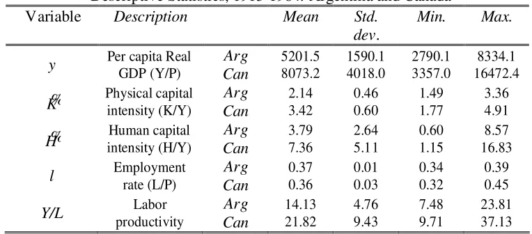
and Obstfeld (2001), Crozier (1983) and the CANSIM database. Table 1 shows univariate
statistics, including the mean, standard deviation, minimum and maximum of all variables.
TABLE 1
Descriptive Statistics, 1913-1984. Argentina and Canada
Variable Description Mean Std.
dev.
Min. Max.
y Per capita Real GDP (Y/P) Arg Can
5201.5
8073.2 1590.1 4018.0 2790.1 3357.0 16472.4 8334.1
K% Physical capital intensity (K/Y) CanArg 2.14 3.42 0.46 0.60 1.49 1.77 3.36 4.91
H% intensity (H/Y) Human capital CanArg 3.79 7.36 2.64 5.11 0.60 1.15 16.83 8.57
l Employment rate (L/P) Arg Can
0.37
0.36 0.01 0.03 0.34 0.32 0.39 0.45
Y/L Labor
productivity
Arg Can
14.13 21.82
4.76 9.43
7.48 9.71
23.81 37.13
Table 2 and Table 3 show correlations between pairs of variables. In the case of Argentina,
income per capita appears strongly correlated with labor productivity and human
capital-product ratio. Capital-capital-product ratio shows also high correlation with income per capita, but
more detailed analysis shows that correlation is stronger, but not linear (see scatter diagrams in
[image:28.595.108.490.445.613.2]look at the scatter diagram shows that negative correlation coefficient emerges from later
observations (i.e. 1976 and after), when employment rate fell below 35% and product grew
much faster than population. Before that period, the relationship between both variables seems
to be positive.
TABLE 2
Argentina. Correlation figures
Y K% H% L Y/L
Y 1.000
K% 0.835 1.000
H% 0.978 0.908 1.000
L -0.692 -0.773 -0.720 1.000
Y/L 0.995 0.855 0.978 -0.755 1.000
TABLE 3
Canada. Correlation figures
y K% H% L Y/L
Y 1.000
K% 0.398 1.000
H% 0.950 0.527 1.000
L 0.685 0.182 0.606 1.000
Y/L 0.977 0.380 0.938 0.520 1.000
In the case of Canada, capital-output ratio shows a weak correlation coefficient with product
per capita. A careful look of the scatter plot shows that after the 1940s a positive and higher
relation between them prevails. Before that period the relation between both series becomes to
negative23. In the case of human capital-product ratio, the correlation is high and positive but
only for highest levels of per capita income; in lower per capita product values the relation
becomes more instable. Something similar occurs with employment rate and per capita income;
at higher levels of income, employment rate increases parallel with per capita product. The
relationship becomes negative in middle range income figures and turns back to be positive
(but at a lesser slope) in lower levels of per capita income. These patterns alert us about a
structural break in Canadian economy near 1940s that altered economic aggregates. This
23 This relationship could be explained by the conjunction of some effects: the last phase of strong capitalization in
breakpoint also matches up with the period of acceleration of the gap between Argentina and
Canada.
Table 4 exhibits the sources of the explanatory variables used in the second stage –i.e. the
explanation of the developing gap- and gives some descriptive statistics. We proceed to
estimate a linear model for explaining the divergence path between Argentina and Canada.
Instead of takingϕ•i, only the numerator of its expression is considered as the dependent
TABLE 4
Sources and descriptive statistics, 1913-1984. Argentina and Canada V ariable Sources and
description Mean Std. dev. Min. Max.
Roughly indicators of social infrastructure: Public expenditure
(GOV)
Ferreres (2005) and McInnis (2004); Public
expenditure/GDP Arg Can 21.7 15.1 7.9 6.6 7.9 6.8 45.4 41.6 Inflation (CPI)
Ferreres (2005) and CANSIM; Ln(CPI 1999=100) Arg Can -23.8 2.7 4.6 0.6 -27.3 1.8 -8.5 4.2 Infant Mortality Rate
(IMR) Abouharb & Kimball (2005)
Arg Can
78.4
59.8 30.8 49.7 30.0 8.0 138.0 186.3
Polity (POL)
Variable “Polity 2” of Gleditsh’s Polity IV
Data Archive††
Arg Can -2.8 9.9 5.8 0.3 -9.0 9.0 8.0 10.0 Index of Democratization (DEM) Vanhanen (2002)’s Polyarchy Dataset Arg Can 7.1 20.4 8.8 5.2 0.0 7.2 29.9 29.3 Political Regime (REG) Banks dataset; Argentine Regime
Dummy† 0.7 0.5 0 1
Integration status: Openness 1
(OPE)
IEERAL (1986) and McInnis (2004); X plus
M/GDP
Arg Can
0.4
0.4 0.3 0.1 0.1 0.2 1.0 0.6
Openness 2 (DUT)
Ferreres (2005), Bird (1985); Customs Duties
on total Budgetary Revenue Arg Can 0.3 0.2 0.2 0.2 0.0 0.0 0.6 0.6
T erms of Trade (TOT)
Ferreres (2005), Wilkinson (1985) and
CANSIM; ln(TOT 1971=100)
Arg Can
4.5
4.6 0.2 0.1 4.1 4.4 4.9 4.7
US TFP index (UST)
Véganzonès and
Winograd (1998) 757.3 219.1 435.8 1071.2
International interest rate
(IIR)
Ferreres (2005);
Short-term UK interest rate 4.5 3.5 0.5 15.1
Geography:
Wheat production (WHE)
Ferreres (2005) and CANSIM; Wheat production (000, ton)
Arg Can 6434.9 12967.2 2188.1 5393.9 2100.0 4389.2 15000.0 26714.7 Beef exports (BEE)
Ferreres (2005), Trant (1985) and CANSIM;
Beef exports (000, ton) Arg Can 554.4 28.3 156.8 24.6 230.3 0.7 981.2 104.5 Natural resources abundances (NRA) IEERAL (1986), Crozier (1985) and CANSIM; Primary activities/GDP Arg Can 0.2 0.1 0.1 0.1 0.1 0.0 0.5 0.3 †
See text for details. †† Previous to the regression process, we added 10 units to each figure of the
5. Empirical results
5.1. Decomposing the development gap24
We calibrate the production function keeping α =0.30 and β =0.28 (1-α-β =0.42) as did it
Mankiw et al (1992) and Klenow and Rodriguez-Claire (1997). Véganzonès and Winograd
(1998) used the same α for a comparative historical study between Argentina and United
States. Blyde and Fernández-Arias (2005) used a capital income share of 1/3 but their
sensibility analysis showed no qualitative differences in the results when they use capital share
of 0.4 or 0.5. Manuelli (2005) mentioned that the analysis of the individual Latin American
country studies suggest values of α ranging from 0.3 to 0.7 and cites Gollin (2002)’s advice
about adjusting downward the estimate of the capital share because problems in measurement.
Katz et al. (2007) compute the participation of labor in the Argentine product following
Gollin’s methodology and achieve the value of 0.52 for our 1-α-β parameter. However, they
specify a production function without human capital, and both models do not totally
comparable and this value is not directly applicable. Hence, although we recognize some
possible bias coming from model specification or measurement problems, the selected
parameters and the later sensibility analysis let us to think that its magnitude is low.
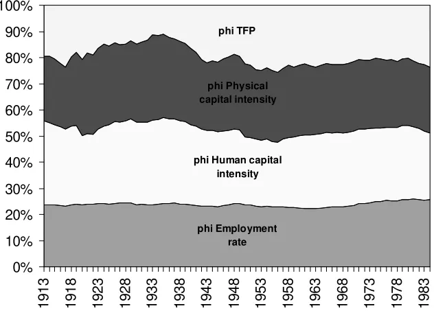
Figure 2 shows the decomposition of the relative per capita GDP between Argentina and
Canada during the period, that is the evolution of index ϕ•i25. Roughly, factor accumulation
explains 80% of per capita GDP differences between Canada and Argentina over 1913-1984.
Nevertheless, technological differences are not a minor source of per capita GDP differences,
24 For convenience purposes, Canadian figures are placed in numerator, thus a fall (rise) in any ratio above 1
means convergence (divergence) between both economies. While a fall (rise) in any ratio down on 1 means divergence (convergence) between both economies.
25 For convenience purposes, expressions in (4) were transformed multiplying the arguments of the logarithms of
accounting between 11 and 26%. The most relevant feature is that the relative importance of
[image:33.595.147.463.183.411.2]both aspects changed over time.
Figure 2. Decomposition of relative per capita GDP between Argentina and Canada
phi Employment rate phi Human capital
intensity phi Physical capital intensity phi TFP 0% 10% 20% 30% 40% 50% 60% 70% 80% 90% 100% 1 9 13 1 9 18 1 9 23 1 9 28 1 9 33 1 9 38 1 9 43 1 9 48 1 9 53 1 9 58 1 9 63 1 9 68 1 9 73 1 9 78 1 9 83
It is clear that there are at least four sections on the figure of the indexes. The ϕAi reduces its
magnitude during a first phase (1913-35), then it increases substantially until 1956 (second
phase) and drop again toward the same standard as the beginning of the first phase. Finally, the
year 1980 starts a new phase with an increasing relevance for relative TFP . Lower values of ϕAi
mean that TFP gap was lower than per capita GDP one. Conversely, the increases in ϕKi and
ϕHi must be interpreted as signals of increasing divergence in physical and human
capital-product ratios. The first and third phases matched that characterization. In contrast, during the
second and fourth phases TFP , although behind factor accumulation, is gaining importance
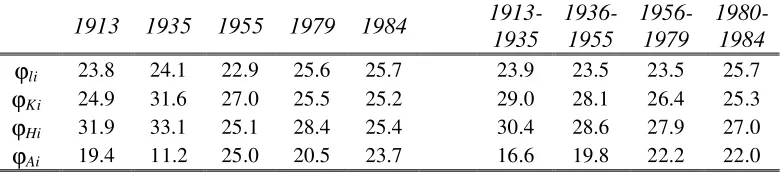
compared to fixed investment for per capita GDP gaps explanation. Table 5 demonstrates this
description. Both annual dates and period averages tell a similar story: during the phase of
TFP decreased its contribution to income gap. After that, when divergence between both
economies tends to consolidate, TFP gap increased its weight26.
TABLE 5
Decomposition of the relative per capita GDP between Argentina and Canada
1913 1935 1955 1979 1984 1913-1935
1936-1955
1956-1979
1980-1984 ϕli 23.8 24.1 22.9 25.6 25.7 23.9 23.5 23.5 25.7
ϕKi 24.9 31.6 27.0 25.5 25.2 29.0 28.1 26.4 25.3
ϕHi 31.9 33.1 25.1 28.4 25.4 30.4 28.6 27.9 27.0
ϕAi 19.4 11.2 25.0 20.5 23.7 16.6 19.8 22.2 22.0
Periodization follows major breakdowns registered above.
Considering gaps in per capita GDP , factor accumulation and TFP evolution, our results show
that Canadian take-off with respect to Argentina, started at mid-1930s. The sources of that
structural change must be placed on a decline in Canadian capital-product ratio counterweighed
by improvements in global efficiency. In contrast, Argentina boosted physical capital intensity
at the expense of efficiency and technology upgrading. Argentina’s experience illustrates that
capacity expansion (not only in equipment, but also in workers´ formal education) must be
accompanied by growing technological competences; otherwise inefficiencies would arise and
per capita income stagnates or decline over time. These results are consistent with Véganzonès
and Winograd (1998). They find a relatively low efficiency of the Argentine economy after
1933 with a slower adoption of foreign technological progress and weaker diffusion.
Figure 3 shows the behavior of the Canadian, Argentine and relative TFPs for the benchmark case,
forthcoming Model 1.
26 Sanz Villarroya (2005) found econometrically the chronological point of break in the convergence path in 1936
[image:34.595.107.497.160.246.2]Figure 3. Canadian (thin line), Argentine (thick line) and relative (triangles) TFPs: Model 1 0 2000 4000 6000 8000 10000 1 9 13 1 9 18 1 9 23 1 9 28 1 9 33 1 9 38 1 9 43 1 9 48 1 9 53 1 9 58 1 9 63 1 9 68 1 9 73 1 9 78 1 9 83 c oun try 0 0,2 0,4 0,6 0,8 1 1,2 1,4 re la ti ve
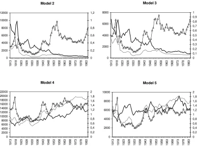
Figure 5. Canadian (thin line), Argentine (thick line) and relative (triangles) TFPs: Model 2-5
[image:35.595.101.503.405.714.2]Figure 5 shows the same lines for different values of parameters of the production function. For
Model 2 we use α =0.30 and β=0.40 resulting 1-α-β =0.30. Model 3 is computed using α =0.40 and β =0.28 and 1-α-β =0.32. Model 4 and model 5 are considered extreme because the very
low participation of human capital on product. For the first one we use α =0.30 and β =0.10
resulting 1-α-β =0.69 while for the last we use α =0.50 and β =0.01 resulting 1-α-β = 0.49.
We should note that models one to three tell a story somewhat different of the following. While
they show that Argentine (and Canadian) TFP fell all over the period, it is possible draw an
upward line with models four and five. But, under any estimates of A, TFP gaps between
Argentina and Canada show two clear phases; the former going from 1913 up to early 1930s
where efficiency gap shows a rapid increase in favor of Canada at the beginning and a
downward evolution after where Argentina seems leading in technological terms. The second
period, from early 1930s to 1984, covers the relative take-off of Canadian TFP . Different TFP
estimations show that, besides a similar gap behavior, the levels of relative efficiency differ.
When labor participation is near or above 0.5, Canada surpasses Argentina in TFP . When
factors contribute in similar magnitude, Argentina is rather superior to Canada27.
5.2. Explaining the development gap
As a result of the previous empirical exercise, we proceed to estimate a linear model for
explaining the technological gap. The ratio between technological levels of each
country,ACAN AARG, is considered as the dependent variable. Results are presented in Table 6.
27 It is possible differ some sub-phases; for example, the effects on TFP of the world crises or particular aspects of