Munich Personal RePEc Archive
Risk in the EU banking industry and
efficiency under quantile analysis
Mamatzakis, E and Koutsomanoli, A
University of Piraeus
14 July 2009
Online at
https://mpra.ub.uni-muenchen.de/22492/
Risk in the EU banking industry and efficiency under quantile
analysis
July 2009
Anastasia Koutsomanoli-Filippaki* and Emmanuel Mamatzakis**
Abstract
This study estimates cost efficiency under a quantile regression framework. Our purpose is to investigate whether cost efficiency differs across quantiles of the conditional distribution. Efficiency scores are derived using the distribution-free approach. Results show that for higher conditional distributions, efficiency scores are lower. In a second stage analysis, we examine the relationship between risk, measured as distance to default and efficiency. Cross section regressions show that the higher the risk the lower the level of efficiency. The magnitude and the significance of the coefficient of the distance to default increases for conditional distributions associated with lower levels of efficiency.
JEL Classification: G21; L25
Keywords: Cost efficiency; Quantile regression; Distribution-free approach; Distance
to default.
1. Introduction
The efficiency of the European banking industry has attracted particular research
attention, as is documented by its long tradition in the literature (i.e., Allen and Rai
(1996), Lozano-Vivas et al., 2001, De Guevara and Maudos, 2002, Maudos et al.,
2002, Vander Vennet, 2002, and Casu and Molyneux, 2003). A large number of
studies on bank efficiency has emerged as a result of rapid changes in the structure of
the European financial services industry in response to major advances in regulation
and technology and to the implementation of the EU Single Market and the Monetary
Union. These developments have created a more competitive financial sector
throughout Europe and have spurred research interest in the banking systems of the
European Union. Indeed, in light of the increased competition under the Single
Market for financial services, the ability of EU credit institutions to compete and
survive in an increasingly integrated European financial landscape has become even
more important. This has been convincingly highlighted by the recent financial crisis,
as the emergence of an increasingly integrated financial market in the EU has
increased contagion risks, thereby jeopardizing financial stability (De Larosiere
Report, 2009). Moreover, the different structures and past legacies of the European
countries create additional challenges in terms of real convergence in a unified
European banking market. At the same time, the dominant role played by banks in the
provision of financial services in the European economies makes the performance of
the banking system crucial for economic development and for the sound functioning
of the industrial sectors, as an improvement of bank performance would lead to a
better allocation of financial resources, and therefore to an increase of investment that
The importance of efficiency measures as instruments for the analysis of bank
performance becomes explicit, partly because efficiency scores provide an accurate
evaluation of the performance of individual banks, but also of the financial industry as
a whole, and partly because of the information that efficiency scores entail regarding
the cost of financial intermediation and the overall stability of financial markets.
Several studies have investigated efficiency in the European banking industry, and
particularly focused on cross-country comparisons, using either parametric (i.e., Allen
and Rai, 1996; Altunbas et al., 2001; Bikker, 2002; Carbo et al., 2002; De Guevara
and Maudos, 2002; Maudos et al., 2002; Vander Vennet, 2002) or non-parametric
approaches (i.e., Lozano-Vivas et al., 2001; 2002; Casu and Molyneux, 2003) or both
(Weill, 2004). Overall, one of the main findings of most of these studies is the
existence of significant efficiency differences across EU countries.
However, despite the plethora of studies investigating efficiency in the
European banking industry, this paper departs from previous literature in several
ways. First, we use, for the first time, quantile regression analysis to estimate banks’
cost function. This type of analysis, proposed by Koenker and Bassett (1978), allows
us to derive different parameter estimates of the cost function for various quantiles of
the conditional distribution and as a result different efficiency scores. In particular, the
quantile regression relaxes one of the fundamental conditions of the OLS and permits
estimating various quantile functions, examining in particular the tail behaviours of
that distribution.1 Therefore, quantile regression is capable of providing a complete
statistical analysis of the underlying diversity of stochastic relationships among
stochastic variables by supplementing the estimation of conditional mean functions
with an entire family of conditional quantile functions.
1
Secondly, we investigate the relationship between cost efficiency and risk
across different quantiles. This interaction has become particularly important, in light
also of recent adverse events in global financial markets. In particular, the on-going
financial crisis has indentified several shortcomings in the functioning of the global
financial system and specifically, significant incentive misalignments that have
greatly contributed, on the micro level, to the current financial turmoil (Caprio et al.
2008). In essence, these misaligned incentive structures have contributed to an
understatement of true risk, generating mispricing of credit instruments. In light of
this, the quantile regression analysis allows us to examine whether the underlying
relationship between risk and performance changes across quantiles. This is an issue
of particular importance as the recent crisis has demonstrated that the tales of the
distribution, i.e. representing higher risk, may hold the key of understanding what
have been malfunctioned in the banking industry.
Moreover, we measure risk using banks’ distance to default (DD thereafter)
(see Merton, 1974), which is considered to be a more comprehensive indicator of risk
than the commonly used index-number proxies based on accounting data. To
empirically estimate cost efficiency, we follow Berger (1993) and employ the
Distribution-free approach (DFA thereafter). Apart from risk, in a second stage
analysis, we also investigate the relationship between efficiency and other bank
specific and macroeconomic variables.
Overall, we employ the quantile regression methodology to address a number
of questions regarding cost efficiency and risk in the European banking system and
discuss their policy implications. What is the level of cost efficiency across countries
under different quantiles? Is there a general trend that can describe the evolution of
between efficiency and risk and how does this relationship evolve across quantiles?
What is the relationship between efficiency and various banking variables and does
quantile estimation affect these interactions?
A first glimpse at the results shows efficiency scores exhibiting marked
diversity across quantiles that would go unnoticed in the classical efficiency
estimations. In particular, we find that in higher quantiles average cost efficiency is
lower compared to that of lower quantiles. In addition, our analysis regarding the
relationship between risk and efficiency suggests that there is a positive relationship
between efficiency and banks’ distance to default, especially in the case of lower
conditional distributions. Moreover, the second-stage regression analysis reveals that
the interaction between efficiency and various banking and macroeconomic variables
varies substantially across quantiles. Two notable examples are the relationship
between cost efficiency and bank concentration and the relationship between
efficiency and credit risk.
The rest of the paper is organized as follows. Section 2 presents the
methodology, while Section 3 provides the description of the data. Section 4 discusses
the empirical results, while conclusions are drawn in Section 5.
2. Methodology
2.1 Quantile regression
Quantile regression is a statistical technique intended to estimate, and perform
inference about, conditional quantile functions. This analysis is particularly useful
asymmetric, fat-tailed, or truncated distribution.2 In the context of our study, quantile
analysis provides an ideal tool to examine evidence on bank efficiency heterogeneity,
departing from conditional-mean models.
Moreover, let y be a random variable with the distribution function FY and
be a real number between zero and one. The th quantile of FY we denote as qY( )
and is derived as the solution to Fy = , that is
qY( ):= FY 1 ( ) inf y : FY ( y )
This simply implies that 100 th% (100(1- )%) of the probability mass of Y is below
(above) qY( ).
As in the case of the least squares estimator the th quantile of FY is derived by
minimizing an objective function with respect to q, i.e.,
q y
Y q
y
Y y y q dF y
dF q
y ( ) (1 ) ( )
q y
Y q
y
Y y y q dF y
dF q
y ) ( ) (1 ) ( ) ( )
( .
Note that the first order condition of this minimisation problem gives the th quantile
of FY as
q y
Y q
y
Y y dF y
dF ( ) (1 ) ( )
0
2
) ( ) 1 ( ) (
1 FY y FY y
) ( y FY
Now, when Y has the conditional distribution F Y / X ( y ) , with th
quintile be ( ) : 1 ( )
/
/ X Y X
Y F
Q . ( )
/X Y
Q is a function of X and
solves q y X Y q y X Y
q y q dF ( y ) (1 ) y q dF ( y )
min / /
The conditional medina is thus
) 5 . 0 ( / X Y Q
of F Y / X . Now, taking
) (
/ X Y Q
is a linear function X’ with unknown parameter then the above
min is equivalent to
'
/ '
/ ( ) (1 ) ' ( )
' min X y X Y X y X
Y y y X dF y
dF X
y
The solution gives which is the th conditional quantile
' )
(
/ X
Q Y X
.
Given the above, a quantile regression involves the estimation of conditional
quantile functions, i.e., models in which quantiles of the conditional distribution of the
Hallock, 2000). Briefly stating standard formulation, the linear regression model takes
the form:
i it
it x
y (1)
where (0, 1), xi is a K × 1 vector of regressors, xi denotes the th sample
quantile of y (conditional on vector xi), and i is a random error whose conditional
quantile distribution equals zero.
In general, the objective function for efficient estimation of corresponding to
the th quantile of the dependent variable (y) can be expressed by the following
minimization problem:
i i i
i i y x
i i x
y i
i
i x y x
y
n : :
) 1 ( 1
min (2)
which is solved via linear programming. Note that the median estimator, that is,
quantile regression estimator for = 0.5, is similar to the least-squares estimator for
Gaussian linear models, except that it minimizes the sum of absolute residuals rather
than the sum of squared residuals.
2.2 Estimating cost efficiency
A number of different approaches have been proposed in the literature for the
estimation of bank efficiency, each of which has its individual strengths and
weaknesses (see Berger and Humphrey 1997 for a review). In this study we opt for a
parametric methodology and employ the Distribution-free approach (DFA), developed
by Berger (1993), who follows Schmidt and Sickless (1984). This approach is a
particularly attractive technique due to its flexibility as it does not impose a-priori any
DFA methodology assumes that the inefficiency of each financial institution remains
constant across the sample period and that random error averages out over time.3
By averaging the residuals to estimate bank-specific efficiency, DFA estimates
how well a bank tends to do relative to its competitors over a range of conditions over
time, rather than its relative efficiency at any one point in time (DeYoung, 1997). This
is useful in the banking sector, since relative efficiencies among different banks may
shift somewhat over time because of changes in management, technical change,
regulatory reform, the interest rate cycle, and other environmental influences.4
However, the rationality of the DFA assumptions depends on the length of period
studied.5 Empirical investigation (i.e., DeYoung, 1997; Mester, 2003) into the number
of years that may be needed to strike a balance between the benefits from having an
additional observation to help average the random error and the costs associated with
adding extra information, which increases the likelihood that the efficiency in the
extra year might drift further away from its long term level shows that a six year
period reasonably balances these concerns.
For the estimation of the Distribution-free approach we opt for the translog cost
function6, which gives us the following specification:
3
In detail, the formal procedure used to carry out the separation between inefficiency and the random error can be described in three steps. First, a consecutive series of annual cost functions are estimated for a given set of banks and some predetermined number of years. Secondly, based on this estimated function, the difference between the observed cost and the predicted cost is calculated for each bank, and for each period. Finally, for each bank, the persistent components observed during the sample period are identified and for each bank, the resulting time series of estimated residuals is averaged across time so as to separate cost inefficiency from the annual random errors.
4
According to Berger and Humphrey (1997) the DFA approach gives a better indication of a bank’s longer-term performance by averaging over a number of conditions, than any of the other methods, which rely on a bank’s performance under a single set of circumstances. Therefore, under DFA a panel data is required and only panel estimates of efficiency over the entire time interval are available.
5
Choosing a too short period, may leave large amounts of random error in the averaged residuals, in which case random error would be attributed to inefficiency. On the other hand, if too long a period is chosen, the firm’s average efficiency might not be constant over the time period because of changes in environmental conditions making it less meaningful (DeYoung, 1997).
6
lnCi = 0 +
i
i
i P
a ln +
i
i
Y
ln
i + ½
i j
i ij P Pj a ln ln +½
i j
j ijln iln
+
i j
j i ijlnPln +
i
i iln +½
i
ijln ln
j j i N N + i j j i N Pln ln ij ! i j j i N Y ln ln ij
" + kDi lnvi +ln ui (3)
where all variables are expressed in natural logs.7 Cit denotes observed total cost for
bank i, Pi is a vector of input prices Yj is a vector of bank outputs, and N is a vector of
fixed netputs8. Moreover, because structural conditions in banking and general
macroeconomic conditions may generate differences in banking efficiency from
country to country, we also include country effects in the estimation of the cost
frontier. Note that ui is the bank specific efficiency factor and vi is the random error
term. All elements of Equation (3) are allowed to vary across time with the exception
of ui, which remains constant for each bank by assumption. In the estimation, the lnvi
and ln ui terms are treated as a composite error term, i.e., ln ˆi lnvˆi lnuˆi. Once
estimated the residuals, ln i , are averaged across T years for each bank i. The
averaged residuals are estimates of the X-efficiency terms, ln ui , because the random
error terms, lnvi, tend to cancel each other out in the averaging. Thus, bank’s i
efficiency is defined as:
)] ˆ ln ˆ exp[(ln ) ˆ exp[(ln ) ( ˆ exp[([ )] ˆ exp[(ln ) ( ˆ exp[ min min i i i i i i
i u u
u y p f u y p f
EFF (4)
where lnuˆiis the residual vector after having averaged over time and lnuˆm in is the
most efficient bank in the sample.
that despite the latter’s added flexibility, the difference in results between these methods appears to be very small.
7
To ensure that the estimated cost frontier is well behaved, standard homogeneity and symmetry restrictions are imposed:
i i
a 1,
i ij
a 0,
i
ij 0, i
ij 0
! , im = miand jk= kj, #i,j,k,m.
8
3. Data description
Our data comprises of all listed banks over the period 2000 to 2005 in fourteen
European Union Member States, namely: Austria, Belgium, Denmark, France,
Germany, Greece, Ireland, Italy, Luxembourg, Netherlands, Portugal, Spain, Sweden
and the UK. Balance-sheet and income statement data were obtained from the
Bankscope database, while for the estimation of bank default risk, stock price data
were obtained from the combination of Datastream, Bloomberg and Bankscope
databases. After reviewing the data for reporting errors and other inconsistencies, we
obtain a balanced panel dataset of 690 observations, which includes a total of 115
different banks. The number of banks varies widely across countries, ranging from 3
in Luxembourg to 34 in Denmark.
For the definition of bank inputs and outputs, we follow the intermediation
approach proposed by Sealey and Lindley (1977.9 The output vector includes loans
(defined as total loans net of provisions) and other earning assets, while total cost is
defined as the sum of overheads (personnel and administrative expenses), interest, fee,
and commission expenses. Regarding input prices, the price of labour is proxied by
the ratio of personnel expenses to total assets, while the price of deposits is defined as
the ratio of interest expenses to total funds. We also specify physical capital and
equity as fixed netputs. The treatment of physical capital as a fixed input is relatively
standard in efficiency estimation (Berger and Mester, 1997)10, while the level of
9
A variety of approaches have been proposed in the literature for the definition of bank inputs and outputs; yet, there is little agreement among economists as what unequivocally constitutes an acceptable definition, mainly as a result of the nature and functions of financial intermediaries. See Berger and Humphrey (1992) for a review of the various methods used to define inputs and outputs in financial services.
10
equity is included so as to account for both the risk-based capital requirements and the
risk-return trade-off that bank owners face (Färe et al., 2004). Apart from this, a
bank’s capital directly affects costs by providing an alternative to deposits as a
funding source for loans (see Berger and Mester, 1997).
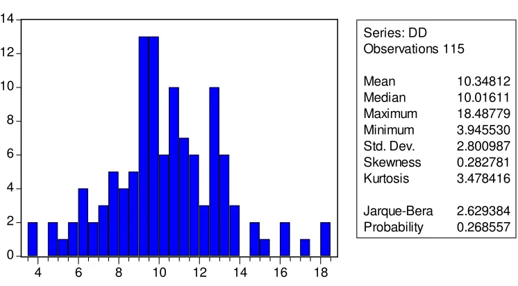
The methodology for the computation of bank default risk is presented in the
Appendix (Appendix A). The annual equity volatility for each bank is estimated based
on the daily returns, derived as the standard deviation of the moving average of daily
equity returns times 261 . All liabilities are assumed to be due in one year, T=1,
while as the risk free interest rate we take the twelve months interbank rate, except for
Greece, for which we opt for the six month interbank rate due to data availability.
Liabilities are derived from Bankscope Fitch IBCA and include the total amount of
deposits, money market funding, bonds, and subordinated debt.
(Please insert Table 1 about here)
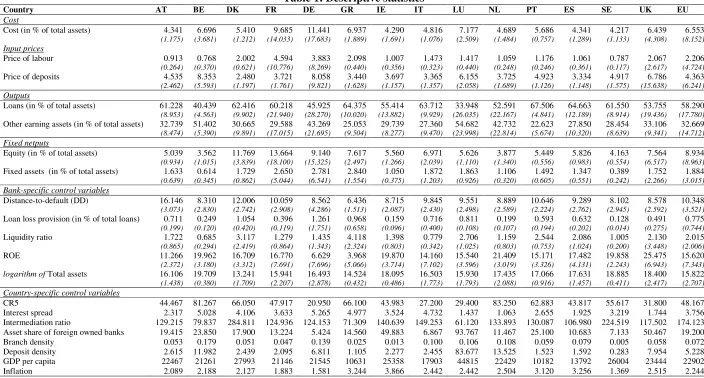
Table 1 provides descriptive statistics of the main variables used in this study
by country and for the overall sample over the period 2000-2005. Overall, there are
considerable variations across countries in relation to cost, outputs quantities and
input prices, as well as differences regarding the size of the country-specific control
variables.
4. Empirical results
4.1 Cost efficiency under a quantile regression analysis
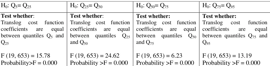
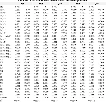
The estimated parameters of the translog cost function for quantiles 0.05, 0.25, 0.5,
0.75 and 0.95, are presented in Appendix B. These estimates have been obtained using
estimation of the entire variance-covariance matrix, which allows us to test the
hypothesis of whether the coefficients between different quantiles are equal.11 Table 2
presents the test results for the various quantiles. All tests show that coefficients are
statistically different from each other between all quantiles, confirming the validity of
our analysis.
(Please insert Table 2 about here)
Next, we calculate cost efficiency scores for each bank in our sample using the
Distribution-free approach and compare these scores across quantiles and across
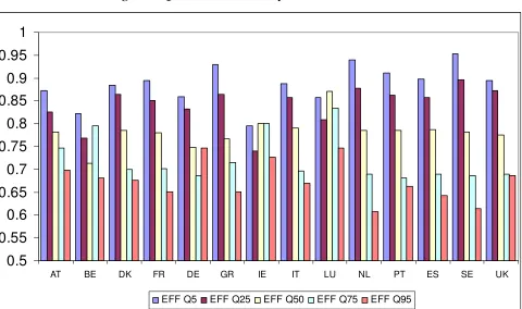
countries. Figure 1 presents the average efficiency scores by country across quantiles (
0.05 to 0.95).
(Please insert Figure 1 about here)
Overall, we observe a marked variability between the average efficiency
scores across quantiles, suggesting that previous research on efficiency, which is
based on the approximation of the mean function of the conditional distribution,
delivers an incomplete notion of the efficiency dispersion across banks. In particular,
the average efficiency score for the whole sample ranges from 0.68 for quantile 0.95
to 0.88 for quantile 0.05. More importantly, cost efficiency estimates across quantiles,
and particularly in the tail of the distribution, differ substantially from the conditional
mean (OLS) point estimate of efficiency, as it is approximated by quantile 0.5. This
suggests that the quantile regression analysis clearly provides a more comprehensive
picture of the underlying range of disparities in cost efficiency that the classical
estimation would have missed.
Moreover, note that a distinct common pattern emerges across quantiles. In
particular, we observe that average efficiency follows a negative trend at higher order
11
of quantiles, indicating the existence of monotonically decreasing quantile efficiency.
In particular, cost efficiency is estimated at around 0.88 for quantile 0.05, drops to
0.85 for quantile 0.25, declines further to 0.78 and 0.71 for quantiles 0.50 and 0.75
respectively, while it reaches its minimum value at 0.68 when the cost function is
calculated at the 0.95 quantile. Nevertheless, this observed pattern between average
efficiency and quantile conditional distributions is less clear in the cases of Germany
and the UK. In particular, the average cost efficiency for German banks drops from
0.85 for quantile 0.05 to 0.68 for quantile 0.75, but rises to 0.74 when the cost
function is estimated at the 0.95 quantile. Similarly, in the case of the UK, average
cost efficiency drops from 0.89 at quantile 0.05 to 0.68 at quantile 0.75, while it
remains stable when the cost function is estimated at the 0.95 quantile. Overall,
efficiency scores exhibit however a negative trend at higher quantiles for the majority
of countries, that is, average efficiency decreases for the upper tail of the distribution.
(Please insert Table 3 about here)
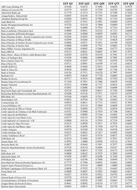
To shed more light into our analysis, Table 3 presents the estimated cost
efficiency scores for each bank in our sample across different quantiles. Overall,
Table 3 reveals a similar picture to the one of Figure 1, and confirms our previous
finding of a negative trend of efficiency scores across higher quantiles. In particular,
for the vast majority of banks in our sample, efficiency scores decrease as the cost
function is estimated at higher quantiles. Yet, there are some notable exceptions,
concerning mostly German and British banks. Note, for example, DAB Bank,
Deutsche Bank, HSBC Trinkaus & Burkhardt AG, Irish Life & Permanent Plc, LBB
Holding AG, Man Group Plc and Oldenburgische Landesbank (OLB), which present
the most notable exceptions. Moreover, Dexia, Fortis, Irish Life & Permanent Plc,
that is higher in quantile 0.95 compared to quantile 0.75. In the case of IKB Deutsche
Industriebank AG cost efficiency is higher in the upper tail of the distribution,
quantile 0.75, compared to quantile 0.5. These findings may be of some interest in the
aftermath of the recent credit crisis as Dexia and Fortis were among the banks that
came close to default, whereas IKB closed hedge funds in 2007 as a result of the
experienced large losses linked to the downturn in the U.S. mortgage market. Given
that for these banks the classical estimations underestimate their underlying
inefficiency scores, quantile analysis appropriately identifies the true disparity of
efficiency scores across conditional distributions, which in turn would be of crucial
importance for the performance, and ultimately for the survival of banks.
4.2 Cost efficiency and risk
The previous section has showed that the disparity of efficiency scores across
conditional distributions would prove critical for appropriately assessing the
performance of financial institutions. In this section, we go a step further and examine
the relationship between cost efficiency and risk, as measured by the distance to
default, focusing mainly on the evolution of this interaction across quantiles. The link
between efficiency and risk has long been at the centre of academic research (see for
example, Berger and DeYoung, 1997; Mester, 1996; Hughes, 1999; Hughes et al.,
2001; Altunbas et al., 2000), while the current financial crisis has further highlighted
the shortcomings and inadequacies of risk management models based on Basel II and
has stressed the need to re-appraise the relationship between risk and performance.
Figure 2 shows in scatter plot the relationship between the estimated average
cost efficiency scores for all banks in our sample and four categories of DD scores.
distance-to-default as follows: the first category includes the riskiest banks in the sample, with
estimated DD scores ranging from 0 to 6, while the second riskier group of banks has
DD scores ranging from 6 to 8. The majority of financial institutions in our sample
belongs to the next two categories, with DD scores ranging from 8 to 10.34 and from
10.35 to 13 respectively. Lastly, the least risky banks in our sample are grouped in the
fifth category that have distance-to-default scores higher than 13.12 Overall, and
despite some extreme cases, Figure 2 shows that the relationship between DD scores
and the average efficiency across countries remains relatively stable for low values of
the distance to default, whereas for higher values of the distance to default a slight
positive trend can be observed. This picture might imply that average quantile
efficiency could be positively linked to the distance to default. However, given that
efficiency scores in Figure 2 present average scores across banks, this heavy
averaging could blur the view of the exact nature of the underlying relationships.
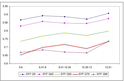
To sharpen the picture, Figure 3 presents efficiency scores under different
quantiles plotted against the distance to default categories defined above. At a first
glimpse, an interesting finding is that for each category of DD scores, average
efficiency levels derived under different quantiles exhibit a clear trend. In detail, the
average cost efficiency at quantile 0.05 is always higher that average cost efficiency at
quantile 0.25 for all clusters of DD scores. Note that in the case of conditional
distributions for low DD scores, that range between 0 to 6, the average cost efficiency
score derived under quantile 0.95 is higher than the average efficiency score of
quantile 0.75. In other words, at the upper tails of the distribution and for low values
of distance-to-default (high default risk), cost efficiency does not follow the negative
trend observed in the case of higher DD scores and lower quantiles.
12
(Please insert Figures 2 and 3 about here)
Nevertheless, the most striking finding derived from Figure 3 is that the
relationship between efficiency and distance-to-default differs not only across the
various quantiles, but also across different levels of default risk. In particular, in both
tails of the distribution of banks’ distance-to-default (banks with the highest and the
lowest default risk), we observe a clear positive relationship between cost efficiency
and distance-to-default across all quantiles. That is, cost efficiency increases for
higher scores of distance-to-default, or in other words for lower levels of risk and this
positive relationship is particularly apparent in the case of the riskiest and the safest
banks in our sample.
On the other hand, the relationship between cost efficiency and
distance-to-default for banks that have DD scores that lay around the median of the distribution is
less clear and differs across quantiles. In particular, for banks with DD scores around
the median in our sample we observe a negative relationship between cost efficiency
and banks’ distance-to-default for quantiles 0.05, 0.25 and 0.95. This is however less
clear in the case of quantiles 0.50 and 0.75, as the relationship between cost efficiency
and distance-to-default changes trend for banks with DD scores around the median.
Overall, our results suggest that while there is some indication of a positive
relationship between cost efficiency and the distance to default for most quantiles and
for most classifications of DD scores, in the case of the 0.5 and 0.75 quantile
distributions and for values of the distance to default from 8.01 to 10.34, cost
efficiency seems to follow a different path. Thus, more analysis is warranted so as to
To this end, we regress banks’ distance to default on cost efficiency derived at
different quantiles. Results are presented in Table 4.13 Despite the fact that only a
small part of the variation in cost efficiency is explained by the distance to default, we
can observe a clear positive relationship between the two variables that increases in
magnitude and significance for higher quantiles, suggesting that a higher level of
efficiency is associated with a higher distance to default and thus with lower risk.
More specifically, whereas for low order quantiles the coefficient of DD is not
significant, for quantiles 0.75 and 0.95 this coefficient becomes highly statistically
significant and also increases in magnitude.
(Please insert Table 4 about here)
This finding suggests that an OLS analysis, which is close to the median
quantile (0.5), would be misleading, as it would report an insignificant coefficient for
the distance to default. On the other hand, quantile regressions by permitting the
estimation of various quantile functions of the underlying conditional distribution
provide us with a more complete picture of the underlying relationships. This is
evident in the present empirical application, where the distance to default appears to
assert a significant and higher in magnitude impact on efficiency for the 0.75 and 0.95
quantiles. Moreover, as we have showed in the previous section, cost efficiency on
average decreases for higher order quantiles (at 0.75 and 0.95) compared to lower
order quantiles. Thus, the positive coefficient of the distance-to-default variable may
suggest that risk asserts a higher impact on banks with low cost efficiency, or
alternatively phrased, banks in quantiles 0.75 and 0.95 are more responsive to risk
than banks placed in quantiles 0.05, 0.25 and 0.5.
13
4.3 Second-stage regressions
As part of a sensitivity analysis we also perform second-stage regressions, where cost
efficiency scores derived at different quantiles are regressed on a set of
macroeconomic and bank variables. In particular, apart from bank’s distance to
default, the following variables are included in our estimations: the capitalization ratio
(E/A) the ratio of loan loss provisions to loans (LLP/L) to control for credit risk, the
liquidity ratio the return on equity ratio (ROE) that captures bank profitability, the
logarithm of total assets (TA) to control for bank size, the ratios of loan to assets
(LO/A) and deposits to assets (DEP/A) that capture banks’ product mix, GDP per
capita (GDPpc) and inflation (INFL) to control for the macroeconomic environment,
the five-firm concentration ratio (CR5) that captures market structure, two measures of
density, the deposits per square kilometre (DEPDEN) and the branches per square
kilometre variables (BRADEN), the intermediation ratio (INTER) that measures
financial development, the interest spread (INTSPR) that captures competition and the
asset share of foreign owned banks (ASFOB). The second stage regressions were
estimated using OLS estimators, where the standard errors were calculated using
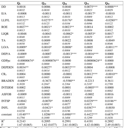
White’s (1980) correction for heteroscedasticity. Table 5 reports the results of the
estimation.14 Overall, several of the coefficients are significant and are in line with our
expectations.
(Please insert table 5 about here)
On the whole, our previous results regarding the relationship between
efficiency and default risk are confirmed. In particular, the sign of the DD coefficient
14
is positive across all quantiles, which implies that the higher the distance to default,
the higher the level of efficiency. Nevertheless, this relationship becomes statistically
significant only for quantiles 0.75 and 0.95, which is consistent with the results
presented in Table 4.
In addition, several interesting results emerge. For instance, we observe that
the least efficient banks, or in other words banks in quantile 0.95, have on average
lower loan loss provisions and a lower ratio of loans to assets. Also banks in quantile
0.95 operate in more concentrated markets and face increased interest spreads. A
similar (though not identical) picture emerges for the 0.75 quantile. In this case, one
can additionally mention the observed negative relationships between efficiency and
the capitalization and liquidity ratios, as well as the deposit ratio. Cost efficiency is
also found to be negatively related to the level of financial development (see
Grigorian and Manole, 2002; Kasman and Yildirim, 2006) and positively related to
the inflation rate. An interesting finding is that the negative relationship between cost
efficiency and market concentration that is reported at 0.95 quantile is reversed at 0.75
quantile. In particular, for banks in quantile 0.75 a higher level of bank concentration
asserts a positive impact on cost efficiency, which indicates that competitive
outcomes are possible even in concentrated systems (Baumol, 1982). This finding
suggests that the relationship between concentration and efficiency is not a
straightforward one, as already suggested by the literature (see for example Casu and
Girardone, 2006) and also that different interactions may exist across different
quantiles and particularly across the most and the least efficient banks in one market.
A similarly mixed picture emerges in the case of the loan loss provisions ratio,
which is reported to assert a positive impact on efficiency at quantiles 0.05, 0.25 and
hypothesis of Berger and DeYoung (1997) could describe more accurately the
behaviour of the worst performing banks, while on the other hand, the relationship
between cost efficiency and the loan loss provisions ratio for banks in higher quantiles
may be better described by the ‘bad management’ or the ‘bad luck’ hypotheses.
According to Berger and DeYoung (1997), the ‘skimping’ hypothesis assumes that
there is a trade-off between short-term costs and future loan performance problems, as
banks that devote fewer resources to credit underwriting and loan monitoring may
appear to be more cost efficient in the short-run. This hypothesis could provide some
explanation on the positive relationship between efficiency and the loan loss
provisions ratio. On the other hand, under the ‘bad management’ hypothesis of Berger
and DeYoung (1997), loan quality is assumed to be endogenous in the quality of bank
management, indicating that managers who are poor at dealing with day-to-day
operations are also poor at managing their loan portfolio, suggesting a negative
relationship between efficiency and the loan loss provisions ratio. This positive
relationship could also be explained by the ‘bad luck’ hypothesis, implying that an
exogenous increase in non-performing loans may force even the most cost efficient
banks to purchase additional inputs necessary to administer these problematic loans
(Berger and DeYoung, 1997). Finally, best performing banks appear to have higher
profitability, a higher fraction of loans in their portfolio, lower branch density and
higher deposit density.
5. Conclusion
This paper investigates cost efficiency in the European banking industry over the
period 2000-2005 using a quantile regression analysis. This type of analysis allows us
and to examine in particular the tailbehaviours of that distribution. This is relevant in
light of the documented heterogeneity in bank efficiency across European countries.
We address several questions related to cost efficiency while we also
incorporate risk in our analysis, in light also of the current re-appraisal of risk
triggered by the global financial crisis. On the whole, we observe significant
differences in the average efficiency across quantiles as well as across countries.
Moreover, bank efficiency exhibits a steady negative trend across quantiles,
suggesting that cost efficiency is higher for lower quantiles of the conditional
distribution compared to higher ones. Also, our analysis suggests that the observed
disparity of efficiency scores across conditional distributions is significant, which
makes the quantile regression estimation a more comprehensive framework for
assessing the performance of financial institutions compared to the classical
estimation.
Regarding the relationship between cost efficiency and risk, our findings
suggest that there is a positive relationship between efficiency and risk, in particular
for higher quantiles. In detail, our results suggest that risk asserts a higher impact on
banks with low cost efficiency, or in other words, banks in quantiles 0.75 and 0.95 are
more responsive to risk than banks placed in quantiles 0.05, 0.25 and 0.5. Moreover,
in a second-stage regression framework, we investigate the relationship between
efficiency and various macroeconomic and banking variables. Our results indicate that
interactions between efficiency and various control variables also vary significantly
across quantiles. Two notable examples are the relationship between cost efficiency
and concentration and the relationship between efficiency and credit risk.
Overall, researchers and policy makers can draw some useful lessons from this
observed heterogeneity in the European banking industry, when examining bank
performance it is important to supplement the estimation of conditional mean
functions with an entire family of conditional quantile functions, so as to get a more
comprehensive picture of efficiency scores. Otherwise, there is a danger of
significantly overestimating banks’ efficiency scores, especially for financial
institutions that are placed at the lower tail of the distribution. In addition, our
findings regarding the relationships between efficiency and default risk, concentration
and credit risk suggest that the interaction between these variables may vary
substantially across quantiles. In other words, the attitude of banks towards risk and
their strategic decisions regarding risk management may well depend on their location
References
Allen, L., Rai, A., 1996. Operational efficiency in banking: an international comparison, Journal of Banking and Finance 20, 655-672.
Altunbas, Y., Gardener, E.P.M., Molyneux, P., Moore, B., 2001. Efficiency in European banking. European Economic Review 45, 1931–1955.
Altunbas, Y., Liu, M-H., Molyneux, P., Seth, R., 2000. Efficiency and risk in Japanese banking. Journal of Banking and Finance 24, 1605-1628.
Bassett, G., Chen, H-L., 2001. Quantile style: return-based attribution using regression quantiles. Empirical Economics 26, 293–305.
Baumol, W.J., 1982. Contestable markets: an uprising in the theory of industry structure. American Economic Review 72, 1-15.
Berger, A., 1993. Distribution-free estimates of efficiency in the US banking industry and tests of the standard distribution assumptions. Journal of Productivity Analysis 4, 261-292.
Berger, A.N., DeYoung, R., 1997. Problem loans and cost efficiency in commercial banks. Journal of Banking and Finance 21, 849-870.
Berger, A., Humphrey, D.B., 1992. Measurement and efficiency issues in commercial banking. In Z. Griliches Eds.: Measurement issues in the services sector, National Bureau of Economic Research, University of Chicago Press, Chicago, 245-279.
Berger, A., Humphrey, D., 1997. Efficiency of financial institutions: international survey and direction of future research. European Journal of Operational Research 98, 175-212.
Berger, A., Mester, L.J., 1997. Inside the black box: what explains differences in the efficiencies of financial institutions? Journal of Banking and Finance 21, 895-947.
Bikker, J.A., 2002. Efficiency and cost differences across countries in a unified banking market. Kredit und Kapital 35, 344–380.
Black, F., Scholes, M., 1973. The pricing of options and corporate liabilities. Journal of Political Economy 81, 637–654.
Caprio, Gerard, Jr., Demirguc-Kunt, A., Kane, E.J., 2008. The 2007 meltdown in structured securitization: searching for lessons, not scapegoats. Policy Research Working Paper No. 4756, The World Bank.
Casu, B., Girardone, C., 2006. Bank competition, concentration and efficiency in the Single European banking market. The Manchester School 74, Special Issue, 441-468.
Casu, B., Molyneux, P., 2003. A comparative study of efficiency in European banking. Applied Economics 35, 1865-1876.
De Guevara, J.F., Maudos, J., 2002. Inequalities in the efficiency of the banking sectors of the European Union. Applied Economics Letters 9, 541-544.
De Larosiere Report, 2009. Report by the high level group on financial supervision in the EU. European Commission.
DeYoung, R., 1997. A diagnostic test for the distribution-free efficiency estimator: An example using US commercial bank data. European Journal of Operational Research 98, 243-249.
Färe, R., Grosskopf, S., Weber, W., 2004. The effect of risk-based capital requirements on profit efficiency in banking. Applied Economics 36, 1731–1743.
Grigorian, D., Manole, V., 2002. Determinants of commercial bank performance in transition: an application of Data Envelopment Analysis. Working Paper No. 2850, The World Bank.
Hughes, J.P., 1999. Incorporating risk into the analysis of production. Atlantic Economic Journal 27, 1-23.
Hughes, J.P., Mester, L.J., Moon, C.-G., 2001. Are scale economies in banking elusive or illusive? Evidence obtained by incorporating capital structure and risk-taking into models of bank production. Journal of Banking and Finance 25, 2169-208.
Kasman A., Yildirim, C., 2006. Cost and profit efficiencies in transition banking: the case of new EU members. Applied Economics 38, 1079-1090.
Koenker, R., 2000. Galton, Edgeworth, Frisch, and prospects for quantile regression in econometrics. Journal of Econometrics 95, 347–374.
Koenker, R. and Bassett, G. 1978. Regression quantile, Econometrica 46, 33–50.
Koenker, R., Hallock, K., 2000. Quantile regression: An introduction. available at http://www.econ.uiuc.edu/~roger/research/intro/intro.html.
Koenker, R., Hallock, K.F., 2001. Quantile regression. Journal of Economic Perspectives 15, 143-156.
Lozano-Vivas, A., Pastor, J.T., Hasan, I., 2001. European bank performance beyond country borders: what really matters? European Finance Review 5, 141–165.
Maudos, J. Pastor, J.M., Perez, F., Quesada, J., 2002. Cost and profit efficiency in European banks. Journal of International Financial Markets, Institutions and Money 12, 33–58.
Merton, R.C., 1974. On the pricing of corporate debt: The risk structure of interest rates. Journal of Finance 29, 449-470.
Mester, L.J., 1996. A study of bank efficiency taking into account risk-preferences. Journal of Banking and Finance 20, 1025-1045.
Mester, L.J., 2003. Applying efficiency measurement techniques to central banks. Working Paper 3-25, Wharton Financial Institutions Centre: Pennsylvania.
Molyneux, P., Altunbas, Y., Gardener, E., 1996. Efficiency in European banking. Chichester: John Wiley & Sons LtD, England.
Schmidt, P., Sickles, R., 1984. Production frontiers and panel data. Journal of Business and Economic Statistics 2, 367-374.
Sealey, C., Lindley, J., 1977. Inputs, outputs and a theory of production and cost of depository financial institutions. Journal of Finance 32, 1251-266.
Taylor, J., 1999. A quantile regression approach to estimating the distribution of multi-period returns. Journal of Derivatives 7, 64–78.
Vander Vennet, R., 2002. Cost and profit efficiency of financial conglomerates and universal banks in Europe. Journal of Money, Credit and Banking 34, 254-282.
Weill, L., 2004. Measuring cost efficiency in European banking: a comparison of frontier techniques. Journal of Productivity Analysis 21, 133–152.
27
Table 1: Descriptive statistics
Country AT BE DK FR DE GR IE IT LU NL PT ES SE UK EU
Cost
Cost (in % of total assets) 4.341 6.696 5.410 9.685 11.441 6.937 4.290 4.816 7.177 4.689 5.686 4.341 4.217 6.439 6.553
(1.175) (3.681) (1.212) (14.033) (17.683) (1.889) (1.691) (1.076) (2.509) (1.484) (0.757) (1.289) (1.133) (4.308) (8.152)
Input prices
Price of labour 0.913 0.768 2.002 4.594 3.883 2.098 1.007 1.473 1.417 1.059 1.176 1.061 0.787 2.067 2.206
(0.264) (0.370) (0.621) (10.776) (8.269) (0.440) (0.356) (0.323) (0.440) (0.248) (0.246) (0.361) (0.117) (2.617) (4.724)
Price of deposits 4.535 8.353 2.480 3.721 8.058 3.440 3.697 3.365 6.155 3.725 4.923 3.334 4.917 6.786 4.363
(2.462) (5.593) (1.197) (1.761) (9.821) (1.628) (1.157) (1.357) (2.058) (1.689) (1.126) (1.148) (1.575) (15.638) (6.241)
Outputs
Loans (in % of total assets) 61.228 40.439 62.416 60.218 45.925 64.375 55.414 63.712 33.948 52.591 67.506 64.663 61.550 53.755 58.290
(8.953) (4.563) (9.902) (21.940) (28.270) (10.020) (13.882) (9.929) (26.035) (22.167) (4.841) (12.189) (8.914) (19.436) (17.780)
Other earning assets (in % of total assets) 32.739 51.402 30.665 29.588 43.269 25.053 29.739 27.360 54.682 42.732 22.623 27.850 28.454 33.106 32.669
(8.474) (5.390) (9.891) (17.015) (21.695) (9.504) (8.277) (9.470) (23.998) (22.814) (5.674) (10.320) (8.639) (9.341) (14.712)
Fixed netputs
Equity (in % of total assets) 5.039 3.562 11.769 13.664 9.140 7.617 5.560 6.971 5.626 3.877 5.449 5.826 4.163 7.564 8.934
(0.934) (1.015) (3.839) (18.100) (15.325) (2.497) (1.266) (2.039) (1.110) (1.340) (0.556) (0.983) (0.554) (6.517) (8.963)
Fixed assets (in % of total assets) 1.633 0.614 1.729 2.650 2.781 2.840 1.050 1.872 1.863 1.106 1.492 1.347 0.389 1.752 1.884
(0.639) (0.345) (0.862) (5.044) (6.541) (1.554) (0.375) (1.203) (0.926) (0.320) (0.605) (0.551) (0.242) (2.266) (3.015)
Bank-specific control variables
Distance-to-default (DD) 16.146 8.310 12.006 10.059 8.562 6.436 8.715 9.845 9.551 8.889 10.646 9.289 8.102 8.578 10.348
(3.073) (2.830) (2.742) (2.908) (4.286) (1.513) (2.087) (2.430) (2.498) (2.589) (2.224) (2.762) (2.945) (2.592) (3.521)
Loan loss provision (in % of total loans) 0.711 0.249 1.054 0.396 1.261 0.968 0.159 0.716 0.811 0.199 0.593 0.632 0.128 0.491 0.775
(0.199) (0.120) (0.420) (0.119) (1.751) (0.658) (0.096) (0.400) (0.108) (0.107) (0.194) (0.202) (0.014) (0.275) (0.744)
Liquidity ratio 1.722 0.685 3.117 1.279 1.435 4.118 1.398 0.779 2.706 1.159 2.544 2.086 1.005 2.130 2.015
(0.865) (0.294) (2.419) (0.864) (1.343) (2.324) (0.803) (0.342) (1.025) (0.803) (0.753) (1.024) (0.200) (3.448) (2.006)
ROE 11.266 19.962 16.709 16.770 6.629 3.968 19.870 14.160 15.540 21.409 15.171 17.482 19.858 25.475 15.620
(2.372) (3.180) (3.312) (7.691) (7.696) (5.066) (3.714) (7.102) (3.596) (3.019) (3.326) (4.131) (2.243) (6.943) (7.343)
logarithm of Total assets 16.106 19.709 13.241 15.941 16.493 14.524 18.095 16.503 15.930 17.435 17.066 17.631 18.885 18.400 15.822
(1.438) (0.380) (1.709) (2.207) (2.878) (0.432) (0.486) (1.773) (1.793) (2.088) (0.916) (1.457) (0.411) (2.417) (2.707)
Country-specific control variables
CR5 44.467 81.267 66.050 47.917 20.950 66.100 43.983 27.200 29.400 83.250 62.883 43.817 55.617 31.800 48.167
Interest spread 2.317 5.028 4.106 3.633 5.265 4.977 3.524 4.732 1.437 1.063 2.655 1.925 3.219 1.744 3.756
Intermediation ratio 129.215 79.837 284.811 124.936 124.153 71.309 140.639 149.253 61.120 133.893 130.087 106.980 224.519 117.502 174.123 Asset share of foreign owned banks 19.415 23.850 17.900 13.224 5.424 14.560 49.883 6.867 93.767 11.467 25.100 10.683 7.133 50.467 19.200
Branch density 0.053 0.179 0.051 0.047 0.139 0.025 0.013 0.100 0.106 0.108 0.059 0.079 0.005 0.058 0.072
Deposit density 2.615 11.982 2.439 2.095 6.811 1.105 2.277 2.455 83.677 13.525 1.523 1.592 0.283 7.954 5.228
GDP per capita 22467 21261 27993 21146 21545 10631 25358 17903 44815 22429 10182 13792 26004 23444 22902
Inflation 2.089 2.188 2.127 1.883 1.581 3.244 3.866 2.442 2.442 2.504 3.120 3.256 1.369 2.515 2.244
Table 2: Post estimation linear hypotheses testing
H0: Q5= Q25 H0: Q25= Q50 H0: Q50= Q75 H0: Q75= Q95
Test whether:
Translog cost function coefficients are equal between quantiles Q5 and
Q25
F (19, 653) = 15.78 Probability>F = 0.000
Test whether:
Translog cost function coefficients are equal between quantiles Q25
and Q50
F (19, 653) = 24.62 Probability >F = 0.000
Test whether:
Translog cost function coefficients are equal between quantiles Q50
and Q75
F (19, 653) = 6.23 Probability >F = 0.000
Test whether:
Translog cost function coefficients are equal between quantiles Q75 and
Q95
Table 3: Quantile cost efficiency scores across banks
EFF Q5 EFF Q25 EFF Q50 EFF Q75 EFF Q95
ABN Amro Holding NV 0.9166 0.8514 0.7680 0.6644 0.5979 Alliance & Leicester Plc 0.8779 0.8195 0.7530 0.6785 0.6665 Allied Irish Banks plc 0.7779 0.7275 0.7751 0.7589 0.7029 Amagerbanken, Aktieselskab 0.8593 0.8148 0.7355 0.6448 0.6037 Arbuthnot Banking Group Plc 0.8204 0.8914 0.7901 0.7143 0.8464 Aspis Bank SA 0.8537 0.7931 0.7091 0.6609 0.5974 Baader Wertpapierhandelsbank AG 0.9728 0.9110 0.7800 0.6609 0.5974 Banca Ifis SpA 0.9647 0.8898 0.7934 0.7254 0.6732 Banca Lombarda e Piemontese SpA 0.9069 0.8941 0.8334 0.7313 0.6688 Banca popolare dell'Emilia Romagna 0.9346 0.8960 0.8059 0.6982 0.6713 Banca Popolare di Intra - Societa Cooperativa per Azioni 0.9256 0.9203 0.8426 0.7616 0.7324 Banca Popolare di Milano SCaRL 0.8599 0.8266 0.7731 0.6828 0.6979 Banca Popolare di Sondrio Societa Cooperativa per Azioni 0.8886 0.8521 0.7651 0.6709 0.6302 Banca Popolare di Spoleto SpA 0.8800 0.8498 0.7767 0.6882 0.7021 Banco Bilbao Vizcaya Argentaria SA 0.8280 0.8095 0.7666 0.6773 0.6244
Banco BPI SA 0.9153 0.8651 0.8067 0.7087 0.7072
Banco Desio - Banco di Desio e della Brianza SpA 0.8259 0.8376 0.8338 0.7491 0.7119 Banco di Sardegna SpA 0.9248 0.8806 0.8000 0.7005 0.6939 Banco Espirito Santo SA 0.8838 0.8387 0.7702 0.6795 0.6786 Banco Pastor SA 0.9711 0.8991 0.8199 0.7101 0.6635 BANIF SGPS SA 0.9058 0.8504 0.7633 0.6598 0.6232 Bank of Attica SA 0.9638 0.8895 0.7809 0.7346 0.7043 Bank of Ireland 0.8126 0.7471 0.8120 0.7997 0.6945
Bankinter SA 0.8955 0.8649 0.7738 0.6805 0.6420
Banque de Savoie 0.9717 0.9535 0.8882 0.7934 0.7326 Banque Degroof Luxembourg SA 0.7430 0.7051 0.7406 0.6678 0.6265 Banque Tarneaud 0.9312 0.8688 0.7747 0.6923 0.6565
Barclays Plc 0.8591 0.8806 0.7607 0.6609 0.5974
Bayerische Hypo-und Vereinsbank AG 0.8738 0.8836 0.8013 0.7184 0.8088 Berlin Hyp-Berlin-Hannoverschen Hypothekenbank AG 0.9208 0.8716 0.7571 0.6735 0.6297
BKS Bank AG 0.9198 0.8659 0.7911 0.7481 0.7454
Bonusbanken A/S 0.8852 0.8704 0.7758 0.6962 0.7344 Commerzbank AG 0.8915 0.8811 0.7713 0.6923 0.7893 Concord Effekten AG 0.9728 0.9110 0.7800 0.6609 0.5974 Credit Agricole de l'Ille-et-Vilaine 0.9163 0.8856 0.7753 0.6876 0.6305 Credit Agricole de Toulouse et du Midi Toulousain 0.9351 0.8960 0.7919 0.7106 0.6631 Credit Agricole du Morbihan 0.8288 0.8089 0.7246 0.6565 0.6109 Credit Agricole Loire Haute-Loire 0.8375 0.8135 0.7261 0.6599 0.6236 Credit Industriel et Commercial - CIC 0.8808 0.8136 0.7919 0.7239 0.6667 Credit Agricole Alpes Provence 0.9223 0.8929 0.7871 0.7074 0.6694 Credit Agricole Sud Rhene Alpes 0.8914 0.8499 0.7550 0.6778 0.6332 Credito Artigiano 0.8578 0.8190 0.7426 0.6538 0.6475 Credito Emiliano SpA 0.8515 0.8023 0.7417 0.6492 0.6483 Credito Valtellinese SCarl 0.8771 0.8453 0.7674 0.6671 0.6202
DAB Bank AG 0.4234 0.4286 0.3837 0.3921 0.5974
Danske Bank A/S 0.9592 1.0000 0.9450 0.8318 0.7025 Deutsche Bank AG 0.8957 0.8444 0.7691 0.7077 0.8986 Deutsche Hypothekenbank (Actien-Gesellschaft) 0.9728 0.9110 0.8468 0.8247 0.6780
Dexia 0.8496 0.8015 0.7524 0.8172 0.6190
DiBa Bank A/S 0.8800 0.8622 0.7879 0.7085 0.6950 Djurslands Bank A/S 0.9398 0.9057 0.8208 0.7204 0.6945
DVB Bank AG 0.8454 0.8198 0.7606 0.6949 0.7745
Erste Bank der Oesterreichischen Sparkassen AG 0.7775 0.7266 0.6845 0.6462 0.6065 Espirito Santo Financial Group S,A, 0.9728 0.9110 1.0000 1.0000 0.8662 FB Bank Copenhagen A/S-Forstaedernes Bank A/S 0.8056 0.7925 0.7251 0.6462 0.6293 Fionia Bank A/S 0.8888 0.8607 0.7693 0.6864 0.6672
Fortis 0.6427 0.5910 0.5822 0.6792 0.6383
HBOS Plc 0.8606 0.8813 0.7995 0.7031 0.6460 HSBC Holdings Plc 0.9517 0.9166 0.7996 0.7200 0.6665 HSBC Trinkaus & Burkhardt AG 0.9340 0.9137 0.8153 0.7979 1.0000 IKB Deutsche Industriebank AG 0.6534 0.6585 0.6785 0.6775 0.6648 Irish Life & Permanent Plc 0.7966 0.7438 0.8150 0.8412 0.7816 Jyske Bank A/S (Group) 0.9031 0.8821 0.8196 0.7224 0.6410
Kas Bank NV 0.9498 0.8906 0.7876 0.7168 0.6241
KBC Groupe SA 0.9728 0.9110 0.8028 0.8903 0.7870 Kreditbanken A/S 0.9725 0.9363 0.8513 0.7741 0.7810 LBB Holding AG-Landesbank Berlin Holding AG 0.8734 0.8500 0.7709 0.7130 0.8195 Lloyds TSB Group Plc 0.9641 0.9137 0.8252 0.7265 0.7129 Lokalbanken i Nordsjaelland 0.8880 0.8309 0.7508 0.6762 0.6225 Lollands Bank 0.9143 0.8903 0.8024 0.7286 0.7017 Man Group Plc 0.9728 0.9110 0.7812 0.7013 0.8211
Max Bank A/S 0.7985 0.7930 0.7220 0.6616 0.6427
Merkur-Bank KGaA 0.8492 0.8313 0.7503 0.6609 0.6473 Millennium bcp-Banco Comercial Portugues, SA 0.9390 0.8935 0.8000 0.6756 0.6415 Moens Bank A/S 0.9086 0.8839 0.8040 0.7196 0.7104
Morsoe Bank 0.9128 0.8932 0.7926 0.7081 0.6881
Natexis Banques Populaires 0.8433 0.7997 0.7581 0.6741 0.6225 Noerresundby Bank A/S 0.9539 0.9098 0.8268 0.7441 0.7286 Nordea Bank AB 0.9480 0.9088 0.7909 0.6969 0.6003 Nordfyns Bank 0.7629 0.7776 0.7174 0.6310 0.6164 Nordjyske Bank A/S 0.9565 0.8848 0.8136 0.7339 0.7101 Northern Rock Plc 0.8483 0.7976 0.7324 0.6377 0.5974
Oberbank AG 0.9036 0.8448 0.7704 0.7270 0.7033
Oesterreichische Volksbanken AG 0.7235 0.6829 0.6666 0.6719 0.6120 Oestjydsk Bank A/S 0.8454 0.8238 0.7159 0.6416 0.6321 Oldenburgische Landesbank - OLB 0.9580 0.9285 0.8132 0.7370 0.9503 Ringkjoebing Bank 0.9626 0.9253 0.8403 0.7551 0.7548 Ringkjoebing Landbobank 0.9503 0.9408 0.8579 0.7644 0.7602 Roskilde Bank 0.9088 0.8694 0.7802 0.6809 0.6361 Royal Bank of Scotland Group Plc (The) 0.8666 0.8302 0.7259 0.6587 0.5995 Salling Bank A/S 0.7789 0.7859 0.7165 0.6327 0.6122 San Paolo IMI 0.8553 0.8505 0.8003 0.6891 0.6548 Skandinaviska Enskilda Banken AB 0.9704 0.8780 0.7593 0.6617 0.6104
Skjern Bank 0.8943 0.8726 0.7714 0.6842 0.6457
Societe Generale 0.9508 0.8993 0.8448 0.7718 0.7015 Spar Nord Bank 0.8670 0.8275 0.7497 0.6590 0.6210 Sparbank Vest A/S 0.7604 0.7846 0.7749 0.6679 0.6329 Sparekassen Faaborg A/S 0.9623 0.9671 0.9173 0.8147 0.8117 Standard Chartered Plc 0.9215 0.8808 0.7881 0.6964 0.7113
Swedbank AB 0.9382 0.9023 0.7937 0.6992 0.6321
Sydbank A/S 0.8911 0.8433 0.7591 0.6657 0.6037
Toender Bank A/S 0.8823 0.8683 0.7630 0.6842 0.6550 Totalbanken A/S 0.8853 0.8504 0.7630 0.6837 0.6573 UniCredito Italiano SpA 0.8541 0.8287 0.7578 0.6628 0.6003 Union Financiere de France Banque 0.8223 0.7357 0.7351 0.6609 0.5974 Van Lanschot NV 0.9510 0.8897 0.7983 0.6897 0.6022 Vestjysk Bank A/S 0.8882 0.8498 0.7623 0.6678 0.6271 Vinderup Bank A/S 0.8686 0.8435 0.7389 0.6943 0.7141 Vorarlberger Landes-und Hypothekenbank AG 1.0000 0.9761 0.9871 0.9563 0.8400 Vorarlberger Volksbank 0.9056 0.8610 0.7935 0.7308 0.6844 Vordingborg Bank A/S 0.8230 0.8364 0.7730 0.6993 0.6900
Note: The table presents bank-specific efficiency scores under different quantiles (Q5, Q25, Q50, Q75, Q95), as estimated by
Table 4: Regression results: Cost efficiency and distance to default
Q5 Q25 Q50 Q75 Q95
Coef. St. Err. Coef. St. Err. Coef. St. Err. Coef. St. Err. Coef. St. Err.
DD 0.005 0.004 0.005 0.004 0.005 0.003 0.007** 0.003 0.011*** 0.003
constant 0.824*** 0.048 0.808*** 0.044 0.731*** 0.040 0.614*** 0.037 0.541 0.043
R-sq 0.129 0.160 0.177 0.259 0.271
Note: The table presents coefficient estimates when regressing efficiency scores derived under different quantiles on distance-to-default. Dependent variable: cost efficiency under quantiles 0.05 (Q5), 0.25 (Q25), 0.5 (Q50), 0.75 (Q75) and 0.95
(Q95). Robust standard errors are presented in italics. Country dummies are also included (not shown) *, **, ***, indicate
significance level at 10%, 5% and 1%, respectively.
Table 5: Second-stage regressions
Q5 Q25 Q50 Q75 Q95
DD 0.0018 0.0006 0.0040 0.0075*** 0.0088***
0.0032 0.0030 0.0025 0.0023 0.0029
E/A -0.0008 -0.0011 -0.0011 -0.0017* -0.0010
0.0013 0.0012 0.0010 0.0009 0.0012
LLP/L 0.0332** 0.0275** 0.0176* 0.0066 -0.0280**
0.0132 0.0125 0.0104 0.0096 0.0122
ROE 0.0027** 0.0021* 0.0023** 0.0014 0.0002
0.0013 0.0012 0.0010 0.0009 0.0012
LIQR -0.0048 -0.0043 -0.0062* -0.0053* 0.0017
0.0040 0.0038 0.0032 0.0029 0.0037
TA 0.0025 0.0009 0.0022 0.0008 -0.0049
0.0050 0.0047 0.0039 0.0036 0.0046
LO/A 0.0009* 0.0010* 0.0008* 0.0005 -0.0011**
0.0006 0.0005 0.0004 0.0004 0.0005
DEP/A -0.0009 -0.0007 -0.0013*** -0.0016*** 0.0000
0.0005 0.0005 0.0004 0.0004 0.0005
GDPpc -0.00000674* -0.0000076** 0.0000 0.00000624** 0.0000
0.0000 0.0000 0.0000 0.0000 0.0000
DEPDEN 0.0034** 0.0027* 0.0032*** 0.0004 -0.0008
0.0015 0.0014 0.0012 0.0011 0.0014
CR5 0.0004 0.0000 -0.0001 0.0012*** -0.0010**
0.0005 0.0005 0.0004 0.0004 0.0005
BRADEN -0.606** -0.3673 -0.5580** -0.2213 0.3611
0.3020 0.2847 0.2364 0.2187 0.2789
INTERM 0.0002 0.0004 0.0001 -0.0005*** 0.0000
0.0003 0.0002 0.0002 0.0002 0.0002
ASFOB -0.0009 0.0000 -0.0011 -0.0002 0.0016
0.0011 0.0010 0.0009 0.0008 0.0010
INTSP -0.0042 -0.0070* 0.0052 0.0229*** 0.0186**
0.0098 0.0092 0.0077 0.0071 0.0090
INFL -0.0320 -0.0421* 0.0207 0.0367** -0.0030
0.0250 0.0236 0.0196 0.0181 0.0231
constant 1.0140*** 1.0206*** 0.6980*** 0.4422*** 0.6876***
0.1794 0.1690 0.1404 0.1299 0.1656
R2 0.2143 0.2095 0.2991 0.4191 0.2892
[image:32.612.110.528.236.668.2]FIGURES
Figure 1: Quantile cost efficiency across countries
0.5
0.55
0.6
0.65
0.7
0.75
0.8
0.85
0.9
0.95
1
AT BE DK FR DE GR IE IT LU NL PT ES SE UK
EFF Q5 EFF Q25 EFF Q50 EFF Q75 EFF Q95
[image:33.612.115.530.441.673.2]Note: The horizontal axis describes the range of different quantiles (0.05, 0.25, 0.5, 0.75 and 0.95) and the vertical axis the corresponding average cost efficiency by country, as measured in a scale from 0 to 1.
Figure 2: Average quantile cost efficiency and DD scores.
0.3 0.4 0.5 0.6 0.7 0.8 0.9 1
0 2 4 6 8 10 12 14 16 18 20
Figure 3: Quantile cost efficiency scores across different scores of DD
0.6 0.65 0.7 0.75 0.8 0.85 0.9 0.95
0-6 6.01-8 8.01-10.34 10.35-13
13.01-EFF Q5 EFF Q25 EFF Q50 EFF Q75 EFF Q95