Effect of Correlation Level on the Use of Auxiliary Variable in Double Sampling for Regression Estimation

Effect of Correlation Level on the Use of Auxiliary Variable

in Double Sampling for Regression Estimation

Dawud Adebayo Agunbiade*, Peter I. Ogunyinka

Department of Mathematical Sciences, Olabisi Onabanjo University, Ago-Iwoye, Nigeria Email: *_{[email protected]}

Received June 21, 2013; revised July 21, 2013; accepted July 28,2013

Copyright © 2013 Dawud Adebayo Agunbiade, Peter I. Ogunyinka. This is an open access article distributed under the Creative Commons Attribution License, which permits unrestricted use, distribution, and reproduction in any medium, provided the original work is properly cited.

ABSTRACT

While an auxiliary information in double sampling increases the precision of an estimate and solves the problem of bias caused by non-response in sample survey, the question is that, does the level of correlation between the auxiliary infor- mation x and the study variable y ease in the accomplishment of the objectives of using double sampling? In this re- search, investigation was conducted through empirical study to ascertain the importance of correlation level between the auxiliary variable and the study variable to maximally accomplish the importance of auxiliary variable(s) in double sampling. Based on the Statistics criteria employed, which are minimum variance, coefficient of variation and relative efficiency, it was established that the higher the correlation level between the study and auxiliary variable(s) is, the bet- ter the estimator is.

Keywords: Correlation Level; Auxiliary Variable; Regression Estimator; Double Sampling and Relative Efficiency of

Estimator

1. Introduction

In sampling theory, auxiliary information may be utilized at any of these three stages or by combining two or all of the three stages. These stages are: (1) at the pre-selection stage or designing stage of the survey in stratifying the population; (2) at the sample selection stage; and (3) at the post-selection or estimation stage. In whatever case, the use of auxiliary information in sample survey is bet- ter than the case where no auxiliary information is util- ized. Ratio, regression, product and difference estimators take advantage of auxiliary information at the estimation stage. However, when the population information is not known then double sampling method becomes necessary for estimation. [1] is of the opinion that estimation of re- quired parameters can efficiently be done with ratio and regression methods of estimation with two-phase sam- pling or double sampling method. Double sampling for ratio estimation becomes necessary over double sampling for regression estimation if the data under consideration are well fitted by a straight line through the origin [2]. Among the authors who have recently contributed to the use of auxiliary variable(s) to establish various estimators for the population parameters are [3-5]. However, in both

cases of ratio and regression estimations or the use of double sampling in ratio and regression estimations, there must exists positive correlation between the auxiliary va- riable x and study variable . This article, empirical- ly, investigates to ascertain the importance of correlation level in the use of auxiliary variable in estimating the po- pulation parameter using double sampling for regression estimation method.

y

2. Methodology

2.1. The Regression Estimator Let y x ii, i



1, 2, , n



y

be the sample values of the main character and the auxiliary character x re- spectively obtained with simple random sampling with- out replacement (SRSWOR) of sample size from the population size . The linear regression estimator of the mean as giving by [6] is:

n

N



ˆ l

y  y  X x



(1) where

2

ˆ xy x

S

S

  ; (2)

ˆ _{estimated regression coefficient}

is the population mean;

X

mean of the auxiliary information; an

x

mean of the study variable

y

The mean square error (MSE) of yl is giving as:

 

1 2 2 2 ₂

l y x

f

V y S S S

n  



 _

_{ }  

 xy

  

  (3)

Similarly, the estimated mean square error (MSE) of l

y is giving as:

 

1 2 2 2

ˆ ˆ ₂ˆ

l y x

f

V y s s s

n  



 _{ }

_{ }   _

 xy

 

 (4)

expressing Equation (4) in terms of correlation coefficient; (where ˆ ˆ y

x

s

s

  )

 

1 2 2

ˆ _{1 ˆ}

l y

f

V y s

n 



 _{ }

_{ }  _

  (5)

2.2. Double Sampling for Regression Estimator The When double sampling for regression estimation is to be used, then there must exist non-zero interception of the regression line on the study variable axis of the scat- tered diagram. The double sampling linear regression es- timator of population mean is giving as





ˆ

dl

y  y  xx (6)

where

ˆ estimated simple linear regression coefficient

 

sample mean at the first phase

x 

Reference [7], hence, presented the estimated variance of ydl as

 

2 2 2 2

ˆ

1 1 1 1 _{ˆ ˆ}

2

dl

y y x

V y

s s s

n N n n  

    

xy

s 

 

_{ }  _ _  _   _

 

   

 

(7)

Equation (7) can be expressed in terms of ˆ (where

ˆ _ˆ y x

s

s

 

 

 

 ), this gives

 

1 1 2 1 1 2

ˆ _{1 ˆ}

dl y y

V y s s

n N n n 

    _{  }

_{ }  _ _  _{ }  _

 

   



2 



 (8)

Similarly, [7] presented the optimum variance of dou- ble sampling regression estimator as:

 

2





2









2

0

1

y dl opt

S

V y C C

C

 _

    

 2  (9)

 

2





2





 

2

0

1

ˆ y ˆ

dl opt

s

y c c

c

V     

 

2.3. Correlation Coefficient and Coefficient of Determination

The simplest method for measuring the relationship exis- tence between two variables (one dependent variable and one independent variable) is with the tool of correlation and regression analysis [8]. Correlation coefficient deter- mines the degree of relationship between variables. It is linear when all parts



x yi, i



on a scattered diagram seem

to lie near a straight line or it is nonlinear when all parts seem to lie near a curve. This work focuses on linear cor- relation. Correlation between variables can be measured with the use of different indices (coefficients). The three most popular of these indices are: Pearson’s Product-mo- ment correlation, Spearman’s rank coefficient and kan- dall’s tau coefficients. Kendall’s tau established by [9] can be used as an alternative to spearman’s rank correla- tion coefficient for ranked data. [10] analysed the proper- ties of kendall’s coefficient and states that “the coeffi- cient we have introduced provides a kind of average measure of the agreement between pairs of numbers (“agreement”, that is to say, in respect of order) and thus has evident recommendation as a measure of the concor- dance between two rankings” and “In general,  is an easier coefficient to calculation than  . We shall see... that from most theoretical points of view  is prefer- able to )”. It should be noted that Kendall uses  to represent Spearman’s rank correlation coefficient and

 as Kendall Tau correlation coefficient. [11] declared that nowadays the calculation of Kendall’s coefficient posses no problem. Kendall’s coefficient is equivalent to Spearman’s rank coefficient in terms of the underlying assumptions, but they are not identical in magnitude, since their underlying logic and computational formulae are quite different. Similarly, Kendall’s coefficient and spearman’s rank correlation coefficient imply different in- terpretations. [12,13] examined the use of Pearson’s pro- duct moment correlation coefficient and Spearman’s rank correlation coefficient for geographical data (on map data that are spatially correlated).

2

ˆ 

 (10)

interval scales. [14] confirmed that Pearson’s product- moment correlation coefficient (represented with r) was the first formal correlation measure and it is still the most widely used measure of relationship.

The idea of this paper is to use correlation coefficient to determine the level of relationship between the auxil- iary and study variables, after which such data will be analysed with double sampling for regression type esti- mator to know which correlation level significantly con- tributes to the objective of implementing auxiliary vari- able. However, having considered all the correlation co- efficient measures, this paper will use Pearson’s product- moment correlation coefficient.

2.4. Pearson’s Product—Moment Correlation Coefficient and Its Coefficient of

Determination

Pearson first developed the mathematical formula for this important measure in 1985















1

1 2

2 2

1 1

n

i i

i

n n

i i

i i

x x y y r

x x y y



 

 



 _{ }













1

(11)

[12] presented correlation in Equation (11) as the “func- tion of raw scores and mean”. Equation (11) describes r as the Centred and standardized sum of cross-product of two variables. Using the Cauchy-Schwartz inequality, [15] claim that it can be shown that the absolute value of the numerator is less than or equal to the denominator, there- fore, . [14] further presented Pearson Product- moment correlation coefficient as standard covariance. The correlation coefficient is a rescaled covariance and presented as;

1  r

xy

x y

s r

s s

 (12)

where

xy

s Sample covariance of x and y

x

s = Sample standard deviation of x

y

s

When the covariance is divided by two standard devia- tions, the range of the covariance is rescaled to the inter- val between −1 and +1, thus the interpretation of correla- tion follows as in the case of Equation (11).

= Sample standard deviation of y

Correlation is sometimes criticized as having no clini- cal interpretation or meaning [16]. This criticism is miti- gated by taking the square of the correlation coefficient which is often called COEFFICIENT OF DETERMI- NATION. [17] expressed coefficient of determination

 

2

r proportion of common variation in the two vari- ables (that is the “strength” or “magnitude” of the rela- tionship). He emphasized that it is important to know this magnitude or strength in order to evaluate the correlation

between variables. The square index is interpreted as pro- portion of variation in one variable accounted for by dif- ferences in the other variable. According to [16],















2

2 1

1 2

2 2

1 1

n

i i

i

n n

i i

i i

x x y y

r

x x y y



 

 

 

 

  

 _{ } 

_{ } 

 







(13)

Or

2

2 xy

x y s r

s s

 

  

 

  (14) where ₁ 2 ₀.

r

 

Error and Interpretation in Correlation Coefficient

Most common error associated with correlation and re- gression analysis, as emphasized by [16], is confusing when interpreting correlation coefficient result. The most common error in correlation coefficient interpretation is to conclude that changes in one variable causes changes in the other. Correlation coefficient indicates that char- acteristics vary together or in opposite direction. How- ever, not interpreting the results of Correlation coeffi- cient is another common error. [16] claims that the coef- ficient must be interpreted in light of the relationship under study and [18] has given different ways to interpret and estimate for coefficient of determination, though bas- ed on theory dependent.

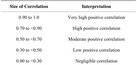
For the purpose of this investigation, this article will make use of the interpretation criteria established by [19] (as seen in Table 1) but with boundary amendment (as in Table 2).

3. Comparison of Estimators

[image:3.595.312.541.130.259.2]

This section proposes on how the empirical comparison will be executed. Minimum variance, coefficient of vari- ation and relative efficiency are the statistical measures that will be used to compare the estimated variance and

Table 1. Correlation coefficient interpretation as presented by [19].

Size of Correlation Interpretation

0.90 to 1.0

(−0.90 to −1.0) Very high positive (negative) correlation 0.70 to 0.90

(−0.70 to −0.90) High positive (negative) correlation 0.50 to 0.70

(−0.50 to −0.70) Moderate positive (negative) correlation 0.30 to 0.50

(−0.30 to −0.50) Low positive (negative) correlation 0.00 to 0.30

[image:4.595.57.287.111.221.2]

Table 2. Correlation coefficient interpretation proposed for this investigation.

Size of Correlation Interpretation

0.90 to 1.0 Very high positive correlation

0.70 to <0.90 High positive correlation

0.50 to <0.70 Moderate positive correlation

0.30 to <0.50 Low positive correlation

0.00 to <0.30 Negligible correlation

the standard deviation of double sampling for regression type estimator at three levels of correlation coefficient which will be termed as high, moderate and low positive linear correlation coefficients (see Table 2 for the details

on the correlation coefficient).

3.1. Coefficient of Variation (CV)

Coefficient of variation is a statistical measure that will be used to know the level of variability in each of these levels of correlation coefficients. [2] defines the coeffi- cient of variation of an estimator

 

y as the measure of relative variability. Mathematically, it is presented as;

 

SE y

 

CV y

y

 (15)

where y = Sample mean; SE y

 

= Standard Error of

the estimator y; and y0.

The estimated Coefficient of Variation is the standard error expressed as a percentage of the mean.

 

_{ }

 

dl dl

dl

V y CV y

y

 (16)

This can also be presented as;

 

_{ }

 

dl

dl

dl

SE y CV y

y

 (17)

In this article, Equation (16) will be used for the com- putation of the coefficient of variation at different levels of the correlation coefficient after which a tabular com- parison will be made.

3.2. Relative Efficiency

Relative Efficiency is another statistical measure that will be used to measure the efficiency of one estimator over another. The relative efficiency of estimator “a” to esti- mator “b” is expressed as;

 

 

Var

*100% Var

ab

b RE

a

 (18)

3.2.1. Relative Efficiency of High Positive Linear Correlation to Medium Positive Linear Correlation

This measures the efficiency of double sampling for re- gression estimator with high positive linear correlation coefficient to double sampling for regression estimator with medium positive linear correlation coefficient. This is presented as:

 

 

medium

1

high

Var

*100% Var

b RE

a

 (19)

3.2.2. Relative Efficiency of High Positive Linear Correlation to Low Positive Linear Correlation

This measures the efficiency of double sampling for re- gression estimator with high positive linear correlation coefficient to double sampling for regression estimator with low positive linear correlation coefficient. This is pre- sented as:

 

 

low

2

high

Var

*100% Var

b RE

a

 (20)

3.2.3. Relative Efficiency of High Positive Linear Correlation to Low Positive Linear Correlation

This measures the efficiency of double sampling for re- gression estimator with high positive linear correlation coefficient to double sampling for regression estimator with low positive linear correlation coefficient. This is presented as:

 

 

low

3

medium

Var

*100% Var

b RE

a

 (19)

4. Empirical Comparison

This research work uses primary data obtained from five hundred and seventy four (574) questionnaires distrib- uted to the staff and students of Nursing school, Periope- rative Nursing School, School of mid-wifery and Occu- pational Health School, all in University College Hospi- tal (UCH) in Oyo state of Nigeria. The double sampling uses the household monthly average expenditure (in thou- sands of Naira) on food consumption as the study vari- able

 

y and the household size as the auxiliary vari-

able

 

x . The double sampling obtains the first and se-

cond sample sizes at five different levels as presented below. n is the sample size at first phase and is the

sample size at the second phase.

n

It will be observed in Table 3 that the minimum pro-

portion is obtained at n 120 and n40. Hence,

120 and 40

n  n are the optimum sample sizes for

[image:5.595.311.538.83.247.2]

Table 3. Summary of the first and second phase sample sizes at different levels.

Level 1 2 3 4 5

n 140 130 120 100 80

n 50 45 40 35 30

n n 0.3571 0.3462 0.3333 0.3500 0.3750

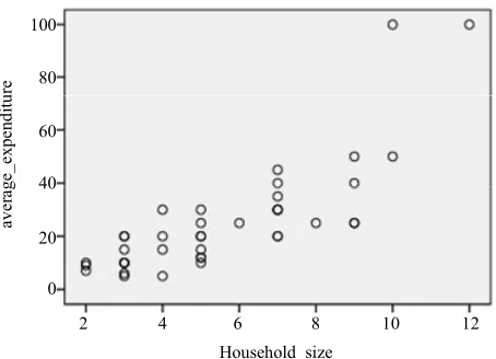
4.1. At High Positive Correlation

Where there exists high positive correlation, Figure 1

shows the existence of positive linear relationship be- tween the auxiliary and the study variables at n 120

SPSS software was used to perform simple linear regression analysis on the data, the model obtained is presented in Equation (22) below.

and n40.

ˆ 10.8820 6.524

y   xe (22) And the Pearson’s Product-moment Correlation Coef- ficient is obtained as and the Coefficient of determination is obtained as . From Equation 22 and Figure 1, this means that the intercept on

axis is not zero; hence, these data are suitable for double sampling for regression type estimation. Similarly, the result of the correlation coefficient shows that of the variation in the household expenditure



79.1% r

2 r 63%

y

63%



y is ex-

plained by the household size

 

x . N 574, n 120,

, 40

n 25.4325 s2 44

7913 dl

.4205

y  , y , ,

,

1.9769 2

x 6.5026

s

42

xy

s   0. and  6.5237.

Using Equation (8), V yˆ

 

dl 5.6671 and the corres-

ponding standard error is SE y

 

_dl 2.3806.

4.2. At Medium Positive Correlation

Where there exists medium positive correlation, Figure 2

shows the existence of approximately positive linear re- lationship between the auxiliary and the study variables at and . SPSS software was used to perform simple linear regression analysis on the data, the model obtained is presented in Equation (23) below.

120

n  n40

ˆ 4.218 5.480

y   x e (23) And the Pearson’s Product-moment Correlation Coef- ficient is obtained as and the Coefficient of determination is obtained as . From Equa- tion (23) and Figure 2, this means that the intercept on

axis is not zero, hence, these data are suitable for double sampling for regression type estimation. Similarly, the result of the correlation coefficient shows that of the variation in the household expenditure

60.8% r

2

r 36.9%



y



y is explained by the household size

 

x . N 574 , n120 ,

40

n , y_dl 26.0154, s2y 441.9769, , 2

sx 5.4333

29.7769

xy

s  ,  0.6076 and  5.4804. Using

2 4 6 8 10 12

Household_size

aver

ag

e_

ex

pe

nd

itur

e

[image:5.595.58.286.110.181.2]

0 20 40 60 80 100

Figure 1. Scatter plot of y against x at high correlation level.

2 4 6 8 10

Household_size

ave

rag

e_

a

ver

ag

e_

ex

pe

nd

itur

e

(0

00

)

0 20 40 60 80 100

Figure 2. Scatter plot of y against x at high correlation level.

Equation (8), V yˆ

 

dl opt 7.5596 and the corresponding

standard error is SE y

 

dl 2.7495.

4.3. At Low Positive Correlation

Where there exists medium positive correlation, Figure 3

shows the existence of approximately positive linear re- lationship between the auxiliary and the study variables at n 120 and n40. SPSS software was used to

perform simple linear regression analysis on the data, the model obtained is presented in Equation (24) below.

1.478 4.745

y   x e (24) And the Pearson’s Product-moment Correlation Coef- ficient is obtained as r42.9% and the Coefficient of

determination is obtained as . From Equation (24) and Figure 3, this means that the intercept on

axis is not zero, hence, these data are suitable for double sampling for regression type estimation. Similarly, the result of the correlation coefficient shows that of the va- riation in the household expenditure



2

r 18.4%

y



y is explained

[image:5.595.311.538.280.433.2]

40

n , y_dl 25.2132, s_y2 511.4045, s2_x 4.1788,

19.8288

xy

s  ,  0.4289 and  4.7451. Using Equ-

ation (8),

 

_dl 10.3260

opt

y 

ˆ

V and the corresponding

standard error is SE y

 

_dl 3.2134.

Summary of the various computations at the three cor- relation levels is presented in Table 4.

4.4. Computation of the Coefficient of Variation As proposed in Equation (17), the coefficient of variation for each correlation coefficient level is obtained and in- terpreted in Table 5.

2 4 6 8 10

household_size

aver

age_

ex

pen

di

tu

re

[image:6.595.60.287.249.406.2]

0 20 40 60 80 100

[image:6.595.57.288.460.585.2]

Figure 3. Scatter plot of y against x at low correlation level.

Table 4. Summary of the different estimated variances at three different correlation levels.

Level High Correlation

Medium Correlation

Low Correlation

n 120 120 120

n 40 40 40

ˆ

 79.1% 60.8% 42.9%

dl

y 25.4335 26.0154 25.2132

  ˆ

dl

V y 5.6671 7.5596 10.3260

 dl

SE y 2.3806 2.7495 3.2134

Table 5. Summary of the different estimated variances at three different correlation levels.

Level High Correlation

Medium Correlation

Low Correlation ˆ

 79.1% 60.8% 42.9%

dl

y 25.4335 26.0154 25.2132

 dl

SE y 5.6671 7.5596 10.3260

Coefficient of

Variation 9.4% 12.3% 14.6%

CV Interpretation _precision Highest _precision Higher _precision High

4.5. Computation of the Relative Efficiency

4.5.1. Relative Efficiency of High Positive Linear Correlation Coefficient to Medium Positive Linear Correlation Coefficient

Using Equation (19):

 

 

medium

1

high

1

Var

*100% Var

7.5596

*100% 133% 5.6671

b RE

a

RE



 

(25)

4.5.2. Relative Efficiency of High Positive Linear Correlation Coefficient to Low Positive Linear Correlation Coefficient

Using Equation (19):

 

 

low

2

high

2

Var

*100% Var

10.3260

*100% 182% 5.6671

b RE

a

RE



 

(26)

4.5.3. Relative Efficiency of Medium Positive Linear Correlation Coefficient to Low Positive Linear Correlation Coefficient

Using Equation (19):

 

 

low

3

medium

3

Var

*100% Var

10.3260

*100% 137% 7.5596

b RE

a

RE



 

(27)

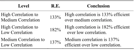
The result obtained for the relative efficiency as de- rived in Equations (25)-(27) are tabulated as seen in Ta- ble 6.

5. Conclusion

This paper examines the effect of correlation level on the use of auxiliary variable in double sampling for regres- sion estimation. The findings revealed that double sam- pling for regression with high correlation coefficient (be- tween the auxiliary and study variables) has the minimum variance



variance 5.6671 ,



hence, is the most effi- cient estimator. Double sampling for regression with me- dium correlation coefficient performs better



variance

Table 6. Summary of the computed relative efficiency.

Level R.E. Conclusion

High Correlation to

Medium Correlation 133%

High correlation is 133% efficient over medium correlation. High Correlation to

Low Correlation 182%

High correlation is 182% efficient over low correlation.

Medium Correlation to

Low Correlation 137%

[image:6.595.59.285.624.737.2] [image:6.595.311.537.654.739.2]



7.5596

 ; while least efficient estimator is double sam- pling for regression with low correlation level



variance

. Thus, the higher the correlation coefficient (between the auxiliary and the study variables) is, the smaller the variance (as seen in Table 4) is. Similarly, it

was discovered that double sampling for regression with high correlation coefficient has the highest precision

; with double sampling for regression with medium correlation coefficient having higher precision



10.3260





CV 9.4%







12

CV 



.3% and finally is double sampling for re- gression with low correlation coefficient having least precision CV 14.6%



. Hence, the higher the correla-

tion coefficient (between the auxiliary and the study va- riables) is, the higher the precision of the estimate (as re- vealed in Table 5) is. Finally, Table 6 revealed the rela-

tive efficiency of double sampling for regression with high correlation coefficient over double sampling for regres- sion with medium correlation coefficient. Similarly, it is the relative efficiency of double sampling for regression with high correlation coefficient over double sampling for regression with low correlation coefficient. Hence, the higher the correlation coefficient (between the auxiliary and the study variables) is, the more efficient the estima- tor is.

Although, auxiliary information in double sampling procedure increases the precision of an estimate, this pa- per, therefore, suggested for researchers to know that the correlation level between the study variable and the aux- iliary variable will contribute to the efficiency of the es- timator under study. In addition, this result can be gener- alised to all sample survey methodologies that use auxil- iary variable to increase the precision of the estimator.

REFERENCES

[1] W. G. Cochran, “Sampling Technique,” 3rd Edition, John Willey and Sons Inc., New York, 1977.

[2] L. S. Lohr, “Sampling Design and Analysis,” 2nd Edition, Brooks/Cole Cengage Learning, 2010, p. 596.

[3] F. C. Okafor and H. Lee, “Double Sampling for Ratio and Regression Estimation with Sub-Sampling the Non-Res- pondents,” Survey Methodology, Vol. 26, No. 2, 2000, pp. 183-188.

[4] B. K. Pradhan, “A Chain Regression Estimator in Two- Pahse Sampling Using Multi-Auxiliary Information,” Bul- letin of the Malaysian Mathematical Sciences Society,

Vol. 28, No. 1, 2005, pp. 81-86.

[5] A. A. Sodipo and K. O. Obisesan, “Estimation of the Po- pulation Mean Using Difference Cum Ratio Estimator with Full Response on the Auxiliary Character,” Research Journal of Applied Sciences, Vol. 2, No. 6, 2007, pp. 769- 772.

[6] P. Mukhopadhyay, “Survey Sampling,” Narosa Publishing House Pvt. Ltd., 2007, p. 256.

[7] F. C. Okafor, “Sample Survey Theory with Applications,” Afro-Orbis Publication Ltd., 2002.

[8] A. Koutsoyiannis, “Theory of Econometrics,” 2nd Edition, Palgrave Publishers Ltd. (Formerly Macmillan Press Ltd.), 1977.

[9] M. G. Kendall, “A New Measure of Rank Correlation,” Bi- ometrika, Vol. 30, No. 1, 1938, pp. 81-89.

[10] M. G. Kendall, “Rank Correlation Methods,” 4th Edition, Griffin, London, 1948.

[11] T. Kossowski and J. Kauke, “Comparison of Values of Pearson’s and Spearman’s Correlation Coefficients on the Same Set of Data,” Quaestiones Geographicae, Vol. 30, No. 2, 2011, pp. 87-93.

[12] R. Haining, “Bivariate Correlation with Spatial Data,” Ge- ographical Analysis, Vol. 23, No. 3, 1991, pp. 210-227. http://dx.doi.org/10.1111/j.1538-4632.1991.tb00235.x

[13] D. A. Griffith, “Spatial Autocorrelation and Sptial Filter- ing” Springer, Berlin, 2003.

http://dx.doi.org/10.1007/978-3-540-24806-4

[14] W. A. Nicewander and J. L. Rodgers, “Thirteen Ways to Look at Correlation Coefficient,” The American Statisti- cian, Vol. 42, No. 1, 1988, pp. 59-66.

[15] F. M. Lord and M. R. Novick, “Statistical Theories of Men- tal Test Scores,” Addison-Wesley, Reading, 1968. [16] M. A. Lang Tom, “Common Statistical Errors Even You

Can Find! Part 4: Errors in Correlation and Regression Analyses,” AMWA Journal, Vol. 20, No. 1, 2005, pp. 10- 11.

[17] N. Shaban, “Analysis of Correlation and Regression Co- efficients of the Interaction between Yildans Come Para- meters of Snap Bears Plants,” Trakia Journal of Science, Vol. 3, No. 6, 2005, pp. 27-31.

[18] D. J. Ozer, “Correlation and Coefficient of Determination,” Psychological Bullentin, Vol. 97, No. 2, 1985, pp. 307- 315. http://dx.doi.org/10.1037/0033-2909.97.2.307