Munich Personal RePEc Archive
Price and Quality Competition
Chioveanu, Ioana
University College London
1 August 2009
Online at
https://mpra.ub.uni-muenchen.de/21647/
Price and Quality Competition
Ioana Chioveanuy
University College London
February 2010
Abstract
This study considers an oligopoly model with simultaneous price and quality choice. Ex-ante homogeneous sellers compete by o¤ering products at one of two quality levels. The consumers have heterogeneous tastes for quality: for some consumers it is e¢cient to buy a high quality product, while for others it is e¢cient to buy a low quality product. In the symmetric equilibrium …rms use mixed strategies that randomize both price and quality, and obtain strictly positive pro…ts. This framework highlights trade-o¤s which determine the impact of consumer protection policy in the form of quality standards.
Keywords: Oligopoly; Price and quality competition; Quality standards JEL classi…cation: L13; L15; L50
1
Introduction
Di¤erences in the quality of groceries or household supplies sometimes stem from packaging or labelling, availability of information, or expert/celebrity endorsements. Some products indicate an improved recipe, added vitamin C, are labelled as healthy living options, or are endorsed by celebrities/experts. Such quality improvements most often do not call for a long term decision. Firms can relatively frequently change the packaging, slightly improve a recipe or arrange for an endorsement, and rivals are unlikely to observe the internal price-quality decision before making their own choices. Furthermore, in these markets consumers are likely to di¤er in their willingness to pay for quality. Building on these observations, this study proposes an oligopoly model where sellers simultaneously compete in quality and price.
More speci…cally, this analysis shows that in the symmetric equilibrium of the price-quality competition model, the …rms randomize on both prices and qualities. In this setting, price and quality dispersion emerges from competition of ex-ante identical sellers in the provision of a homogeneous product. Some important features of this model are the following. Sellers can choose between two levels of quality. All consumers value both qualities, but it is e¢cient for
I am grateful to Ugur Akgun, Mark Armstrong, V. Bhaskar, Ste¤en Huck, and Jidong Zhou for useful
comments.
yDepartment of Economics and ELSE, UCL, Gower Street, London WC1E 6BT, UK, Email:
some consumers to buy a high-quality, and for others to buy a low-quality.1 The sellers know the
valuations for either quality and their distribution in the population, but they cannot distinguish among buyers and, therefore, cannot price discriminate. The sellers o¤er their products at only one of two quality levels.2
In some professional service markets, the providers (e.g., lawyers, consultants, architects) also compete for consumers not only by quoting a price for the service, but also by simultaneously setting a quality level. The …rms are able to provide the same service at di¤erent levels of quality, but often a …rm’s o¤er is not preceded by a negotiation process, so that there is little transparency regarding the alternative qualities that could have been provided (and could have been closer to consumer’s actual needs.) For instance, when economic consulting …rms make a pitch to a customer, they simply submit a price-quality bid without knowing with certainty the exact level of complexity preferred for the project. A …rm seeking professional advice might have a higher or a smaller stake in an ongoing antitrust investigation, and a person seeking legal advice might have a higher or a lower income. Another example of markets where the …rms compete simultaneously over price and quality is the business software one. In this case, a quality level might stem, for instance, from the maintenance service terms. In these markets, corporate customers are likely to value the speed of response more than home users.
In the price-quality competition model, low-quality is always associated with lower prices, and high-quality with higher prices. At equilibrium, there is a positive probability that any one …rm is the sole provider of a given quality and, even though it faces some competition from the other quality, it can charge a price in excess of marginal cost. The di¤erence between the highest (lowest) price for a high-quality product and lowest (highest) price for a low-quality product is equal to the di¤erence in high-end (low-end) consumers’ valuation for the high and low-quality products. Moreover, the symmetric equilibrium leads to positive expected pro…ts for the …rms. Due to the fact that high-end (low-end) consumers can eventually shift to a di¤erent quality, the highest price at which a high-quality (low-quality) is o¤ered is strictly lower than high-end (low-end) consumers’ valuation of the high-quality (low-quality). Low-end consumers obtain a positive net surplus if they purchase a low-quality and, for a nontrivial range of parameters, this is also the case when they buy a high-quality. High-end consumers are left with a positive net surplus regardless of the quality they consume. This contrasts with most price dispersion models where prices equal to consumers’ willingness to pay for the good are charged with pos-itive probability.3 This is the case in Varian (1980) and Rosenthal (1980), for instance, where
homogeneous sellers compete for consumers with identical preferences who di¤er in their search costs. Some buyers have in…nite search costs and shop at random, while the others purchase from the lowest price seller. The expected pro…t of a …rm equals the monopoly pro…t on its locked-in group (i.e., the corresponding share of random shoppers.)
1That is, high-end consumers’ marginal valuation of the high quality exceeds its cost, while the remaining
(low-end) consumers’ marginal valuation of the high quality does not exceed its cost.
2However, the equilibrium characterized in this research is consistent with a market in which the sellers …rst
decide whether to o¤er only one or both qualities, but to put up a menu of qualities they incur a positive cost.
Armstrong and Chen (2009) analyze price and quality competition in oligopoly. In their model, like in the current one, a high-quality is associated with high prices and a low-quality with lower prices. However, they consider consumers with homogeneous tastes for quality who di¤er in their attentiveness to quality (a low-quality is worthless and would not be produced if there were no inattentiveness).4
Other models of price and quality competition consider consumer heterogeneity, but focus on perfectly competitive markets. Wolinsky (1983) analyses a market where the consumers may di¤er in their taste for quality and receive noisy signals of a seller’s quality. He shows that a separating equilibrium where prices fully reveal quality exists under certain conditions. Buyers with homogenous tastes for quality might still di¤er in their knowledge of product quality: while some are fully aware of quality, others are not.5 Along this line, Cooper and Ross (1984) allow
quality-uninformed consumers to have rational expectations about the price-quality relationship. They show that, with U-shaped average cost functions, there exists a rational expectations equilibrium with dispersion in qualities but not in prices.
Most oligopoly models of price and quality competition focus on cases where quality is a long-run variable, while prices can be adjusted in the short-run (see Shaked and Sutton, 1982 for a seminal contribution). They re‡ect the fact that a quality improvement might involve observable changes in the production facility or long-run investments (e.g., R&D). While this is often the case, there are also many markets where a quality update does not call for signi…cant investments or is unlikely to be observed by the rivals prior to price competition. In the latter cases, strategic interaction is better captured by simultaneous price-quality competition.
The price-quality competition model o¤ers a framework for the analysis of quality standards (QS) in oligopoly. Such intervention has been employed in professional service provision either by governmental entities or professional associations to improve market performance.6 However, QS in oligopoly markets received little attention in the economic literature, and the extant analyses focus on instances in which quality choices precede pricing decisions. The impact of QS in this framework is driven by the trade-o¤ between increasing competition and o¤ering consumers the quality they desire, and it pins down the potentially perverse e¤ects of quality regulation. The impact of a relevant QS which would lead to Bertrand competition depends on the underlying market conditions. This study shows that the a QS might reduce both total welfare and consumer surplus. However, depending on the parameter values, a QS might also boost both total welfare and consumer surplus, or harm welfare while bene…ting the consumers. The paper is organized as follows. Section 2 presents the model and the symmetric mixed strategy equilibrium when the market is fully covered. Section 3 discusses quality standards and section 4 concludes. The proofs missing from the text and the characterization of the symmetric equilibrium when the market is not covered are relegated to the Appendix.
4An alternative "rational" interpretation of their model is that some consumers do not mind consuming the
low-quality product.
5Yet another type of consumer heterogeneity is present in Besancenot and Vranceanu (2004), where high-end
consumers are loyal to the high-quality product (they only care for the extra features provided by a high-quality).
2
A Model of Price and Quality Competition
The Framework
Consider a market where N 2 identical suppliers can o¤er an otherwise homogeneous product at two quality levels, a high one (qH) and a low one (qL). The constant marginal cost of
producing the high-quality isc >0;while the one of producing the low-quality is normalized to zero. Sellers simultaneously choose prices and qualities. Each …rm o¤ers only one quality level. There is a unit mass of consumers, each demanding one unit of the product. A fraction 1
of the consumers are willing to pay 1 for the low-quality and 3 for the high-quality, while a
fraction of the consumers has willingness to pay for the low and high-quality equal to 2 and 4;respectively. I assume that 1 >0; 3 > cand i > j fori > j, and refer to the consumers
with a lower (higher) valuation for either quality as "low-end" ("high-end").7 Assume that it
is e¢cient for low-end consumers to buy a low-quality and for the high-end consumers to buy a high-quality product, that is 3 1 < c < 4 2: However, at equilibrium consumers will
purchase the quality which provides the best deal.
In this model, consumers are able to compare all available products both in terms of price and quality before they purchase. Firms know consumers’ valuations for either quality and the market composition, but cannot price discriminate. When = 0 (or = 1), …rms supply the e¢cient quality qL (or qH), compete a la Bertrand, and make zero pro…ts. The remainder of
this paper focuses on 2(0;1):
Lemma 1 For 2(0;1);a) there is no symmetric pure strategy equilibrium; and b) forN 4; there is a family of asymmetric pure strategy equilibria, where at least two …rms choose each quality, low-quality is o¤ered at p= 0 and high-quality at p=c;and all …rms make zero pro…ts. Total welfare and consumer surplus are given by
( 4 c) + 1(1 ): (1)
Armstrong and Chen (2009) present similar results in a model of bounded rationality (inat-tentiveness) with price-quality competition. In their setting, consumers have homogeneous tastes for quality, but a fraction of them do not observe (or assess) quality and (wrongly) believe that all products are of the same (high) quality.8 In the symmetric equilibrium of their model …rms
mix on both qualities and prices. To exploit consumers’ inattentiveness, …rms provide a useless low-quality product with a positive probability. In contrast, in the current model …rms face fully rational consumers and the symmetric mixed strategy equilibrium discussed below is related to heterogeneity in consumers’ tastes.
The Symmetric Mixed-Strategy Equilibrium
For anyN 2, there exists a symmetric equilibrium in which …rms choose both prices and qualities stochastically and make positive pro…ts. The convex hull of the range of prices which
7Note that consumers’ valuations can be derived from Mussa-Rosen preferences.
are assigned positive probability is [p0; p4]; with 0 < p0 < p4 < 4: There are two threshold
prices p1 2 [p0; 1] and p2 2 [c; p4] such that a low-quality product is chosen if p p1 and a
high one ifp p2 > p1:The probability of o¤ering a low-quality product isF(p1) =F(p2) =P.
The discussion in this section focuses on a situation in which the market is fully covered in equilibrium. Appendix A presents a necessary condition for the market to be fully covered for an arbitrary number of …rms. However, for expositional simplicity, this section assumes that the following su¢cient condition holds:
2+ 3 4 3 c
: (2)
This condition guarantees thatp4 3so that regardless of the price draw all consumers buy the
product. A necessary condition for (2) to hold is 3 > 4 2:Finally, note that if 3 4 2;
then p4 > 3 and with a positive probability low-end consumers are excluded from the market.
The analysis of this case is presented in Appendix B.
When (2) holds, the support of the equilibrium price distributions isS = [p0; p1][[p2; p4].9
The boundary prices p2 and p4 satisfy:
p2=p1+ 3 1 and p4 =p0+ 4 2: (3)
The di¤erence between the lowest price at which a high-quality is o¤ered(p2)and the highest
price at which the low-quality is o¤ered (p1) is exactly equal to low-end consumers’ marginal
valuation for quality (that is, the di¤erence between low-end consumers’ valuation for the high-quality and their valuation for the low-high-quality, 3 1). At the same time, the di¤erence between
the highest price at which a high-quality is o¤ered (p4) and the lowest price at which the
low-quality product is o¤ered (p0) is determined by high-end consumers’ marginal valuation for
quality (that is, the di¤erence between high-end consumers’ valuation for the high-quality and their valuation for the low-quality product, 4 2).
Then, notice that the expected pro…ts of a …rm at pricep0 are
(p0) =p0[1 + (P+ 1 F(p0+ 4 2))N 1] =p0[1 + PN 1]: (4)
At this price only a low-quality is o¤ered. Low-end consumers buy for sure at price p0: a
low-quality is never sold at a lower price, and a high-low-quality (for which they are willing to pay at most 3) provides them with a lower surplus even when it is sold at its lowest possible price
(p2). High-end consumers buy at p0 only if all …rms supply a low-quality. Notice that even if
the high-quality is provided at its maximal price (p4) still high-end consumers are indi¤erent
between purchasing the high-quality and buying a low-quality at p0; its lowest possible price
(this happens because 2 p0 = 4 p4). The last equality in expression (4) follows from the
fact that F(p0+ 4 2) =F(p4) = 1:This must be the case because if all …rms had an atom
atp4;then an individual …rm would be strictly better o¤ moving mass to p4 for some small
9When the market is covered in the symmetric equilibrium, the only relevant boundary prices are p
0; p1; p2
>0:10 The expected pro…ts at price p
4 are given by
(p4) =p4 PN 1 = (p0+ 4 2 c) PN 1: (5)
At price p4 only a high-quality is o¤ered. When p4 3; low-end consumers would buy at p4
with probability (1 F(p4))N 1:This is the probability that all suppliers price abovep4 and is
equal to zero.
In the symmetric mixed strategy equilibrium, a …rm is indi¤erent between any two prices which are assigned positive density. Then, from the equilibrium requirement that (p0) = (p4),
it follows that
p0 = ( 4 2 c)
1 P
N 1: (6)
Note that low-end consumers are indi¤erent between buying a low-quality at price p1 and a
high-quality at price p2 (see (3)). In e¤ect, they weakly prefer a low-quality at price p p1
to a high-quality. High-end consumers buy a low-quality at price p1 only if no …rm supplies
a high-quality and all low-quality suppliers price above p1: But, this happens with probability
zero. Formally, the expected pro…t of a …rm charging price p1 is:
(p1) =p1[(1 )(1 F(p1))N 1+ (P F(p1))N 1] =p1(1 )(1 P)N 1:
By the previous argument low-end consumers buy at p2 only if no …rm supplies a low-quality.
High-end consumers buy for sure at pricep2: this is the best high-quality deal they can get and it
provides a higher net surplus than the best possible low-quality deal ( 2 p0 < 4 (p1+ 3 1),
p2< p4). Then, the expected pro…t of a …rm at pricep2 is:
(p2) = (p2 c) + (1 )(1 F(p2))N 1 = (p1+ 3 1 c) + (1 )(1 P)N 1 : (7)
The constant pro…t condition (p1) = (p2) de…nes
p1 = ( 1 3+c)[1 +
1
(1 P)N 1]: (8) Using (6), (8), and the equilibrium requirement that (p0) = (p2);I obtain
1 2 1 3+c 4 2 c
[ + (1 )(1 P)
N 1
(1 ) + PN 1 ] =
P
1 P
N 1
: (9)
Expression (9) implicitly de…nes the probability of choosing a low-quality (P) which is well de…ned.11 If (2) holds, these expressions are su¢cient to characterize the equilibrium strategies.
Proposition 1 If (2) holds and N 2; there exists a symmetric mixed strategy equilibrium where …rms randomize on prices and qualities. Firms choose prices with support S = [p0; p1][
[p2; p4]: The boundary prices p0; p1; p2 and p4 are de…ned by (3), (6) and (8). The atomless
price cdf F(p) is de…ned implicitly by
p[(1 )(1 F(p))N 1+ (P F(p))N 1] =p1(1 )(1 P)N 1 for p0 p p1 and (10)
(p c)[ (P+ 1 F(p))N 1+ (1 )(1 F(p))N 1] = (p4 c) PN 1 for p2 p p4; (11)
1 0This would result in a jump up in demand and only a negligible loss due to the lower price.
1 1The RHS of (9) is increasing inP and ranges from 0to1, while the LHS is positive and decreasing in P;
where P = F(p1) =F(p2) is the probability of choosing a low-quality and is de…ned by (9). A
low-quality product is associated with prices in [p0; p1]and a high-quality product with prices in
[p2; p4]:
In this symmetric mixed strategy equilibrium, …rms o¤er both a low-quality (at a relatively low price) and a high-quality (at a higher price) with positive probability. As a result of this randomization, with a positive probability, each …rm is the sole provider of a given quality and the sellers are able to sustain positive pro…ts. The mixed strategy equilibrium crucially depends on demand heterogeneity: for some consumers it is e¢cient to buy a low-quality, while for others it is e¢cient to buy a high-quality.12
Recall that each …rm chooses only one quality level in this model. Even if …rms could o¤er a menu of (both) qualities at a cost, the equilibrium presented in Proposition 1 would still apply to a game in which …rms …rst decide if to provide just one quality level or both. If …rms o¤ered both qualities at di¤erent prices, they would end up competing a la Bertrand in two separate markets. Then, they would obtain zero pro…ts and be unable to cover the cost of providing both qualities. Similarly, if …rms face some …xed costs of entry, only the mixed strategy equilibrium could support entry.
In the covered market equilibrium presented in Proposition 1, high-end consumers buy a high-quality product if at least one …rm supplies it (which happens with probability 1 PN)
and buy a low-quality product only if all …rms o¤er a low-quality. Low-end consumers buy a low-quality product if at least one …rm supplies it (which happens with probability1 (1 P)N)
and buy a high-quality product only if all …rms o¤er high-quality products. Then, welfare is given by
( 4 c) (1 PN) + 2 PN + 1(1 )[1 (1 P)N] + ( 3 c)(1 )(1 P)N:
Aggregate pro…ts follow from (5) and (6). Consumer surplus equals total welfare minus aggregate pro…ts. Algebraic manipulations lead to the following result.
Corollary 1 If (2) holds, at equilibrium, the expected pro…t of a …rm is
E = ( 4 2 c)(1 +
1 P
N 1) PN 1;
total welfare is
( 4 c) + 1(1 ) ( 4 2 c) PN (c 3+ 1)(1 )(1 P)N; (12)
and consumer surplus is given by
( 4 c) + 1(1 ) ( 4 2 c) PN 1[P+N(1+
1 P
N 1)] (c
3+ 1)(1 )(1 P)N; (13)
where P is implicitly de…ned by (9).
1 2As expected in a model where consumers can correctly assess product quality, at equilibrium there is a
The source of welfare and consumer surplus loss in the covered market symmetric equilibrium in Proposition 1 comes from the fact that with a positive probability consumers buy an ine¢cient quality. With probability one, all consumers buy and obtain a positive net surplus. But, when all …rms o¤er a low-quality (i.e., with probability PN) high-end consumers obtain a surplus of 2;lower than the net surplus of( 4 c)which is their …rst best. Likewise, when all …rms o¤er a
high-quality (i.e., with probability(1 P)N) low-end consumers buy an ine¢ciently low-quality.
Notice that the …rst two terms in expressions (12) and (13) give the …rst best outcome and the last two terms are negative. The term in square brackets in (13) captures the consumer surplus loss due to pricing above marginal cost.
When the market is not covered (that is, forp4 > 3)13, the symmetric equilibrium introduces
a second source of ine¢ciency. In that case, low-end consumers are excluded from the market with a positive probability (i.e., (1 F( 3))N > 0) and obtain zero surplus. Proposition 3 in
Appendix B presents the symmetric equilibrium when the market is not covered.14
The following example illustrates the type of mixed strategy equilibrium presented in Propo-sition 1.15
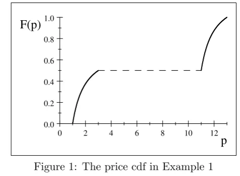
Example 1 Let N = 2; =:5; 1 = 6; 2= 8; c= 10; 3 = 14 and 4 = 20:Using the results
in Proposition 1, at equilibrium, p0 = 1; p1 = 3; p2= 11; p4= 13 andP =:5:The price cdf is
F(p) =
(
:75 :75p for p2[1;3] 1:25 p:7510 for p2[11;13] :
Firms o¤er a low-quality at price p2[1;3]and o¤er a high-quality at p2[11;13]. The equilib-rium pro…t is :75: Consumer surplus is6 and total welfare is 7:5. Figure 1 illustrates the mixed strategy equilibrium in this case.
0 2 4 6 8 10 12
0.0 0.2 0.4 0.6 0.8 1.0
[image:9.595.175.413.493.667.2]p
F(p)
Figure 1: The price cdf in Example 1
1 3Recall that a su¢cient condition to be in this region is
3< 4 2:
1 4Notice that the type of equilibrium which applies depends both on the degree of consumer heterogeneity and
on the number of …rms. When N ! 1; p0!0;and it is possible to have p4 = 4 2+p0> 3 forN < N0
and 4 2< 3 forN N0 for someN0 3:For this reason, the necessary condition for an uncovered market
symmetric equilibrium to exist depends on N:(Appendix A presents a necessary condition for acovered market
symmetric equilibrium to exist for an arbitary number of …rms.)
Large Oligopolies
First notice that whenN ! 1;the probability to choose a low-quality is de…ned by
1 1 3+c 4 2 c
= P 1 P
N 1
,P =
h
1 1 3+c 4 2 c
i1=N 1
1 +h 1 1 3+c 4 2 c
i1=N 1:
Then, limN!1P = 1=2:From (3), (6) and (8), it follows that p0 ! 0 and p2 ! cas N ! 1;
such that the equilibrium cdf in Proposition 1 converges to a discrete distribution which assigns probability 1/2 to p0 and probability 1/2 to p2: In addition, a …rm’s pro…t and total industry
pro…ts both converge to zero when the market is nearly competitive. The outcome of the symmetric mixed strategy equilibrium converges to the asymmetric pure strategy equilibrium of the game presented in Lemma 1: total welfare and consumer surplus in the limit are equal to
( 4 c) + 1(1 ) (see (12) and (13)).
3
Consumer Protection Policy: Quality Standards
The price-quality competition model can be employed to analyze consumer protection policy. This section shows that the impact of a relevant quality standard (QS)16, which would lead to Bertrand competition in the symmetric equilibrium, depends crucially on the underlying market conditions. In a setting of imperfect competition and heterogeneity in consumers’ preferences for quality, a QS is bene…cial for some consumers at the expense of others. Then, the overall e¤ect of such policy on welfare and consumer surplus depends on the composition of the market and on the relative e¢ciency gain of a quality match.
Studies of QS’s in competitive markets with asymmetric information (see Leland, 1979; Shapiro, 1983; and Armstrong, 2008 for a review) have already indicated that some consumer groups might be harmed by the mandatory policy. However, these models do not account for the e¤ects of QS’s on prices. Studies of QS’s under oligopoly price competition (Ronnen, 1991; Crampes and Hollander, 1995) build on the decrease in prices brought about by the policy and conclude that the intervention is always welfare increasing.17 In a duopoly model where …rms …rst choose quality and then prices, and face quality-dependent …xed costs, Ronnen (1991) shows that a QS intensi…es price competition by limiting vertical di¤erentiation and is bene…cial to consumers. Crampes and Hollander (1995) show, in a related duopoly model where the cost of quality is variable, that a QS might decrease consumer surplus. This happens if the increase in the low-quality brought about by the intervention triggers a signi…cant increase in the high-quality.18 In this case, the increase in prices due to higher costs o¤sets the competitive e¤ect. In
1 6A relevant QS lies between the lowest and the highest available quality levels and has a short-run e¤ect on
equilibrium outcomes.
1 7In the case of oligopolyquantity competition, Valletti (2000) shows that QS unambiguously decrease welfare.
1 8In both Ronnen (1991) and Crampes and Hollander (1995), in the unregulated equilibrium, the duopolists
contrast, in my oligopoly model with exogenous quality levels, the impact of a QS depends on the trade-o¤ between the (positive) competitive e¤ect and the (negative) e¤ect of less product diversity, and overall the intervention might reduce welfare.
Notice that, under a relevant QS, welfare and consumer surplus in the price-quality compe-tition model are both given by
WM QS =CSM QS = ( 4 c) + (1 )( 3 c): (14)
A straightforward comparison of the welfare levels in the symmetric free-market equilibrium (12) and under a QS (14) leads to the following result.
Proposition 2 If (2) holds and N 2;a quality standard is welfare decreasing i¤
( 4 2 c) PN <(c 3+ 1) (1 )[1 (1 P)N];
and it decreases consumer surplus i¤
( 4 2 c) PN 1[P +N(1 +
1 P
N 1)]<(c
3+ 1) (1 )[1 (1 P)N]:
Notice that, as N goes to in…nity, the LHS of both inequalities in Proposition 2 converges to zero while the RHS converges to (c 3+ 1) (1 ) > 0: In nearly competitive markets,
a QS harms both consumer surplus and total welfare. The reason is that, in these markets, competition eliminates the price distortion (recall that p0 !0 andp2!c asN ! 1) and the
intervention only restricts consumers’ choice.
Unlike the limit case, in smaller oligopolies the impact of a QS is not clear-cut. For an arbitrary number of …rms, there is no closed-form solution for P; the probability to choose a low-quality in the symmetric equilibrium (see (9)). But, forN = 2;it is possible to calculate P and write the conditions in Proposition 2 in terms of the parameters. This allows to discuss the implication of QS’s for di¤erent parameter regions.
Corollary 2 LetN = 2and b= ( 1 3+c)=( 4 2 c):When (2) holds, a) if = 1=2;then
a quality standard is always welfare decreasing, and it decreases (increases) consumer surplus i¤ b > 3:2 (b < 3:2); b) if b = 1; then a quality standard is always welfare decreasing, and it decreases (increases) consumer surplus i¤ / 0:27 ( ' 0:27); c) if b =
1
2
then for
/0:215 a quality standard raises both welfare and consumer surplus.
consumers whose valuation of the incremental quality imposed by the QS does not cover its cost.19
Figure 2 presents expected welfare and consumer surplus in the symmetric unregulated equilibrium and under a QS: for …xed and i; cranges from8to9:7such thatb(= ( 1 3+
c)=( 4 2 c)) ranges from 0to0:75:
0.0 0.1 0.2 0.3 0.4 0.5 0.6 0.7 5.2
5.4 5.6 5.8 6.0 6.2 6.4 6.6 6.8 7.0 7.2
[image:12.595.188.405.163.336.2]b
Figure 2: Expected welfare (thick line) and consumer surplus (dashed line) in the symmetric equilibrium. Welfare and consumer surplus (thin line) under a MQS.(N = 2; =:2; 1 = 6;
2 = 8; 3= 14; 4 = 20)
Corollary 2 part c) shows that a QS is bene…cial for the consumers and the society when there are few high-end consumers ( small) and the relative e¢ciency gain of quality match to the low-end consumers (captured by b = ( 1 3+c)=( 4 2 c)) is low. When is small,
the probability that all …rms choose a low-quality is higher, and the intervention is more likely to make a di¤erence to the high-end consumers. But, if bis also low, a QS raises both consumer surplus and welfare. This is the case in Figure 2 where = 0:2for low enoughb’s. In this region, the positive e¤ect of a QS on price competition o¤sets its negative e¤ect on product diversity. In contrast, when there are many high-end consumers ( large), p2 (the best high-quality deal)
is close to c and P (the probability of choosing a low-quality) is close to0;so that there is less scope for intervention.
For intermediate values of b the intervention bene…ts consumers, but harms total welfare: in this region, the price e¤ect is strong enough to o¤set the lack of product diversity, but the society is harmed by the quality mismatches. Finally for higher values of b;a QS harms both consumers and welfare: the relative net value of quality to the low-end consumers is high, and the negative impact of reduced variety dominates.
The analysis in this section shows that the impact of consumer protection in the form of QS stems from a trade-o¤ between increasing competition and catering to consumers with di¤erent tastes for quality. Although the intervention increases competition, it also harms consumers
1 9Appendix B focuses on the uncovered market equilibrium and shows that a QS might still decrease welfare
when they place low value on quality.20 Understanding the undesired e¤ects of QS is particularly
important as recent evidence on consumers’ inattention to …ne print terms or shrouded price attributes might make consumer protection policy more appealing. If randomization on quality and prices is driven only by inattention (as in Armstrong and Chen, 2009), a QS is obviously bene…cial. But, my analysis shows that similar market outcomes might stem from heterogeneity in consumers’ tastes for quality. As the presence of few inattentive high-end consumers would not alter qualitatively the equilibrium strategies, with heterogeneous preferences, the e¤ect of a QS meant to protect the inattentives is no longer clear-cut. As a QS forces low-end consumers to purchase an ine¢ciently high-quality product, it might actually harm consumers and welfare overall.21
4
Conclusions
In professional service markets and in some consumer good markets, packaging, labelling, en-dorsements, or maintenance service terms can be used to o¤er better value to buyers. As quality improvements can be made in the short-run and are unlikely to be observed by rivals prior to product market interaction, these situations call for a model of simultaneous price and quality competition. This paper proposed an oligopoly model where ex-ante identical sellers compete in the provision of a product by simultaneously submitting price-quality bids. Each …rm chooses one of two quality levels. The consumers have heterogeneous tastes for quality: it is e¢cient for some consumers to buy a high-quality, while for others is e¢cient to buy a low-quality. In the symmetric equilibrium …rms use mixed strategies that randomize both price and quality, and obtain strictly positive pro…ts.
The analysis of consumer protection in the form of quality standards in this setting captures (undesired) e¤ects neglected by previous models of imperfect competition. The intervention increases price competition, but reduces product diversity.
5
Appendix
Proof of Lemma 1. a) If all …rms choose high (or, low) quality, they compete a la Bertrand and make zero pro…ts. Then, a unilateral deviation to a low (or, high) quality and price p is pro…table as it generates strictly positive pro…ts equal to (1 )" (or, (" c)) whenever
0< p < c ( 3 1)(or,c < p < 4 2). Hence, there is no symmetric pure strategy equilibrium.
2 0Under perfect competition and informational asymmetries, Leland (1979) derives conditions under which QS
increases welfare, but warns that "when entry is restricted in this manner detrimental side e¤ects may occur." While the negative impact of intervention in his setting is the same as here, the positive e¤ect is di¤erent as it
stems from correcting the "lemons problem".
2 1Armstrong (2008, pp. 146-7) introduces inattention (some consumers prefer a high quality, but do not pay
attention to quality) in the perfectly competitive version of this model and shows that a QS meant to protect the inattentive, might be bene…cial or not depending on the parameter values. (In his perfectly competitive model, a
b) If at least two …rms o¤er a low-quality and at least two …rms o¤er a high-quality, all …rms compete a la Bertrand, make zero pro…ts and there is no pro…table unilateral deviation. In this equilibrium, all low-end consumers buy a low-quality at p= 0 and all high-end consumers buy a high-quality atp=c.
5.1 Appendix A: Covered Market Equilibrium
Conditions for the Existence of a Symmetric Covered Market Equilibrium
For expositional simplicity, the main text assumes that (2) holds. This is a su¢cient condition for the market to be covered in the symmetric equilibrium. Let us now derive (2) and present a more complex necessary condition for an arbitrary number of …rms.
First note that the market is covered in the symmetric equilibrium if p4 3; where p4 is
the upper bound of the support of the equilibrium pricing cdf. (Clearly, if p4 > 3 there is
a positive probability that low-end consumers are excluded from the market. This happens if all …rm o¤er high-quality products at prices higher than low-end consumers’ valuation of the high-quality product, 3:) By (3) and (6),
p4= ( 4 2 c)
1 P
N 1+
4 2: (15)
Using the fact thatP <1(see 9), the requirement thatp4 3 leads to the su¢cient condition
(2):
2+ 3 4 3 c
:
To obtain a necessary condition for the market to be covered in the symmetric equilibrium for an arbitrary number of …rms, note thatP(N)is decreasing (see (9)), so thatp4(N)is decreasing.
It follows that p4(N) p4(2):Using (15), p4(2) = ( 4 2 c)1 P(2) + 4 2;where P(2)
follows from (9):
P(2) = b(1 )
2
(2 )+ 2
(1 ) p[b(1 )2(2 )+ 2(1 )]2 4b(1 )2[b(1 )3 3] 2[b(1 )3 3
] ;
where b= ( 1 3+c)=( 4 2 c):Then,p4 3 for any N 2 i¤
b(1 )(2 ) + 3 p[b(1 )(2 ) + 2]2 4b[b(1 )3 3]
2[b(1 )3 3]
3 4+ 2 4 2 c
:
Proof of Proposition 1. ForF(p)de…ned by (10) and (11) to be a well-de…ned cdf, it has to be continuous and increasing onS:Let us …rst consider prices in[p0; p1]:By (10),F is increasing
inp: I show in continuation that F(p0) = 0:Notice that (10) evaluated at p0 gives
p0[(1 )(1 F(p0))N 1+ (P F(p0))N 1] =p1(1 )(1 P)N 1
and using (6) and (8) it becomes
1 2 1 3+c 4 2 c
[ + (1 )(1 P)
N 1
(1 )(1 F(p0))N 1+ (P F(p0))N 1
] = P 1 P
N 1
But from (9) and (16), it follows that F(p0) = 0:
Let us consider prices in [p2; 3]\[p2; p4]:By (11), F is increasing in p: I show in continuation
that F(p2) =P:Notice that (11) evaluated at p2 gives
(p2 c)[ (P + 1 F(p2))N 1+ (1 )(1 F(p2))N 1] = (p0+ 4 2 c) PN 1 ,
(p1+ 3 1 c)[ (P + 1 F(p2))N 1+ (1 )(1 F(p2))N 1] = (p0+ 4 2 c) PN 1
and using (6) and (8) it becomes
1 2 1 3+c 4 2 c
[ (P+ 1 F(p2))
N 1+ (1 )(1 F(p 2))N 1
1 + PN 1 ] =
P
1 P
N 1
: (17)
But from (9) and (17), it follows that F(p2) = P = F(p1): In addition, notice that if p4 =
p0+ 4 2 2[p2; 3]then (11) evaluated atp4 gives
(p4 c)[ (P + 1 F(p4))N 1+ (1 )(1 F(p4))N 1] = (p4 c) PN 1
and it follows that F(p4) = 1:
The boundary price p1 should not exceed 1:Ifp4 3;from (5) and (7), it follows that
p1 = 1 3+c+ (p0+ 4 2 c)
PN 1
+ (1 )(1 P)N 1 1 3+p4 1:
For the strategies presented in Proposition 1 to be indeed an equilibrium, there should be no pro…table unilateral deviation. The relevant deviations to be considered in this case are the following: i. o¤er a low-quality atp2(p1; 1];ii. o¤er a high-quality atp2[c; p2]; and iii. o¤er
a high-quality atp2(p4; 4]:
Notice that deviations with a high-quality on[p0; c]are not pro…table because the price is below
marginal cost and deviations with a low-quality in ( 2; 4] are not pro…table because the price
exceeds the willingness to pay for low-quality. Notice that deviations with a low-quality to some pricep2( 1; 2)\(p1; 2) are not pro…table: Low-end consumers cannot a¤ord the low-quality.
High-end consumers buy only if a high-quality is not o¤ered at this price (i.e., F( 2) F(p2)).
Then, they purchase at p with probability (P F(p) + 1 F(p+ 4 2))N 1 = 0. The last
equality follows from the fact that, in this range, p+ 4 2 > p0 + 4 2 = p4 so that
F(p+ 4 2) = 1 and F(p) =P:
i. The deviator o¤ers a low-quality atp2(p1; 1]:low-end consumers buy atp only if all other
…rms price above 3 1+p. high-end consumers buy at p with probability (P F(p) + 1
F(p+ 4 2))N 1 = 0:Then, deviator’s pro…t is
D(p) =p(1 )(1 F(p+ 3 1))N 1:
As p 2 (p1; 1]; notice that p+ L 2 (p1+ 3 1; 3] = (p2; 3]: Then F(p+ 3 1) is
de…ned by
Notice that, by continuity, D(p1) = p1(1 )(1 F(p2))N 1 = p1(1 )(1 P)N 1 = E:
Using (18), deviator’s price and pro…ts are given respectively by
p=c+ 1 3+ E
[ (1 F(p+ 3 1) +P)N 1+ (1 )(1 F(p+ 3 1))N 1]
and
D(F) =fc+ 1 3+ E
[ (1 F +P)N 1+ (1 )(1 F)N 1]g(1 )(1 F) N 1:
For 3 c < 1; @ @FD(F) < 0 such that D(p) D(p1) = E: Consequently, this is not a
pro…table deviation.
ii. The deviator o¤ers a high-quality at p2[c; p2). Then, his expected pro…t is
D(p) = (p c)[ + (1 )(1 F(p+ 1 3))N 1]:
Clearly, all high-end consumers buy at p. low-end consumers buy only if all other …rms price above p+ 1 3. Asp2[c; p2);(p+ 1 3)2[c+ 1 3; p1):
First let us consider deviations to p such that p+ 1 3 2 [p0; p1): Then, F(p+ 1 3) is
de…ned by
(p+ 1 3)[(1 )(1 F(p+ 1 3))N 1+ (P F(p+ 1 3))N 1] =p1(1 )(1 P)N 1: (19)
By (19), deviator’s price and its pro…t are respectively:
p= 3 1+
p1(1 )(1 P)N 1
(1 )(1 F)N 1+ (P F)N 1 > c and
D(F) =f 3 1 c+
p1(1 )(1 P)N 1
(1 )(1 F)N 1+ (P F)N 1g[ + (1 )(1 F) N 1]:
It can be shown that @ D(F)
@F > 0 (recall that 3 1 c < 0), and then for all p 2 [p0; p1); D(p) D(p2): But, D(p2) = (p2 c) [ + (1 )(1 P)N 1] = E: Consequently, this is
not a pro…table deviation.
Ifc+ 1 3 < p0 for someN;then for anyp2[c+ 1 3; p0];it holds thatF(p+ 1 3) = 0.
It follows that @ D(p)
@p >0 and D(p) D(p0) E as the previous argument applies. (Notice
however that as N ! 1; p0!0;and c+ 1 3>0.)
iii. The deviator o¤ers a high-quality atp2(p4; 4]:Low-end consumers do not buy here (they
strictly prefer a low quality, or a high quality at a lower price), and high-end consumers buy only if deviator’s deal is the best available. For deviations with p2[p4; p1+ 4 2], deviator’s
pro…t is
D(p) = (p c) (P F(p+ 2 4))N 1:
For p2(p4; p1+ 4 2]; p+ 2 42(p0; p1]and F(p+ 2 4) is de…ned by
(p+ 2 4)[(1 )(1 F(p+ 2 4))N 1+ (P F(p+ 2 4))N 1] = E: (20)
By (24), deviator’s price and its pro…t can be written respectively as:
p= 4 2+c+ E
(1 )(1 F)N 1+ (P F)N 1 and D(F) =f 4 2 c+ E
It can be shown that @ D(F)
@F < 0 (recall that 4 2 c > 0);and then in the relevant range D(p) D(p4):Notice that D(p4) = (p0+ 4 2 c) PN 1 = E:Hence, there is no gain
from such deviation. For deviations with p 2 (p1 + 4 2; 4]; neither low-end nor high-end
consumers purchase, so clearly there is no gain from such deviation.
Finally, notice that, as the deviations above are not pro…table, …rms cannot gain from mixing on quality either.
Proof of Corollary 2. a) Let = 1=2:Then, (9) becomes
b(2 P 1 +P) =
P
1 P ,P =
1 + 3b p1 +b(14 +b)
2(1 b) forb6= 1 and P = 1=2 forb= 1:
It can be easily checked that P 2(0;1)forb 2(0;1) with limb!1P = 1:For N 2;a QS is
welfare decreasing if
( 4 2 c)P2 <( 3 1 c) [(1 P)2 1],P <
2b
2b+ 1;
and is consumer surplus decreasing if
( 4 2 c)P[P+ 2(1 +P)]<(c 3+ 1) [1 (1 P)2],P <
2(b 1) 3 +b : The result then follows.
b) Let b= 1:Then, (9) becomes
1 2
[ + (1 )(1 P) (1 ) + P ] =
P
1 P ,
P = (1 )[2(1 )
2+ p(1 2 )2+ 4]
2(1 2 )(1 + 2) if 6= 1=2and P = 1=2 if = 1=2:
It can be easily checked that P 2(0;1)for 2(0;1)withlim !0P = 1 andlim !1P = 0:
A QS is welfare decreasing whenever
P2<(1 )[1 (1 P)2],P <2(1 ); which turns out to be true for all ’s.
A QS is consumer surplus decreasing if P[P + 2(1 +
1 P)]<(1 )[1 (1 P)
2],P < 2(1 2 )(1 )
1 + 2 :
This leads to the result. c) Let b=
1
2
. Then, (9) becomes:
[ + (1 )(1 P) (1 ) + P ] =
P
1 P ,
P = 2(1 ) +
p
5 4 (1 )]
2(1 2 ) for 6= 1=2 and P = 1=2for = 1=2:
It can be easily checked that P 2 (0;1) for 2 (0;1) with lim !1P = 0: First notice that if
a QS raises welfare, then it also raises consumer surplus (see Proposition 2). A QS is welfare increasing whenever
( 4 2 c) P2 >(c 3+ 1) (1 )[1 (1 P)2],P >
2b(1 ) +b(1 ):
5.2 Appendix B: Uncovered Market Equilibrium
In this part, I present the symmetric mixed strategy equilibrium in the uncovered market case. A su¢cient condition for the market to be uncovered is 4 2 > 3:In this case the support of
the price cdf is [p0; p1][[p2; 3][[p3; p4]:Notice …rst that expressions (3)-(9) still apply. To pin
down the equilibrium cdf’s it is necessary to identify the boundary pricep3 and the probability
to price below 3;that is F( 3)<1. These are implicitly de…ned by (5) together with:
( 3) = ( 3 c)[ (P+ 1 F( 3))N 1+ (1 )(1 F( 3))N 1]and (21)
(p3) = (p3 c) (P+ 1 F( 3))N 1:
low-end consumers purchase a high-quality at 3(which leaves them with zero net surplus) only if
this is the lowest price in the market and they no longer purchase it atp3because their valuation
of a high-quality is lower. high-end consumers obtain a higher net surplus from the high-quality sold at 3than from the best possible low-quality deal, that is 4 3> 2 p0 , 4 2+p0 > 3:
Similarly, high-end consumers obtain a higher net surplus from the high-quality sold atp3 than
from the best possible low-quality deal, that is 4 p3 > 2 p0 , 4 2+p0 = p4 > p3:
Hence, they buy at 3 or atp3 if all other …rms o¤er a low-quality or charge a higher price.
Proposition 3 ForN 2and 4 2 > 3;there exists a symmetric mixed strategy equilibrium
where …rms randomize on prices and qualities. Firms choose prices with support S = [p0; p1][
[p2; 3][[p3; p4]:The boundary pricesp0; p1; p2; p3 andp4 are de…ned by (3), (6), (8) and (21).
The atomless pricing cdf F(p) is de…ned implicitly by
p[(1 )(1 F(p))N 1+ (P F(p))N 1] =p1(1 )(1 P)N 1 for p0 p p1;
(p c)[ (P + 1 F(p))N 1+ (1 )(1 F(p))N 1] = (p0+ 4 2 c) PN 1 for p2 p 3; and
(p c) (P + 1 F(p))N 1 = (p0+ 4 2 c) PN 1 for p3 p p4: (22)
where P = F(p1) = F(p2) is the probability of choosing a low-quality de…ned by (9) and p3 is
de…ned by (5) and (21). A low-quality is associated with prices in[p0; p1]and a high-quality with
prices in [p2; p4]:
Proof. As most of the arguments overlap with those presented in the proof of proposition 1, I focus here on the additional arguments required for the uncovered market case.
a) Pricing cdf analysis. Let us consider prices in [p3; p4]which are assigned positive density
ifp4 > 3. By (22),F is increasing inp:I show in continuation thatF(p3) =F( 3):Notice …rst
that from (21), the boundary pricep3 is given by
p3 =c+( 3 c)[ (P + 1 F( 3))
N 1+ (1 )(1 F(
3))N 1]
(P+ 1 F( 3))N 1
If we evaluate (22) atp3 and substitute (23), then it becomes
( 3 c)[ (P + 1 F( 3))N 1+ (1 )(1 F( 3))N 1]
(P + 1 F( 3))N 1
(P + 1 F(p3))N 1=
(p0+ 4 2 c) PN 1:
But, as indi¤erence between 3 and p4 requires
( 3 c)[ (P+ 1 F( 3))N 1+ (1 )(1 F( 3))N 1] = (p0+ 4 2 c) PN 1
it follows that F(p3) =F( 3):
b) Boundary prices. Whenp4> 3;from (7) and ( 3) in (21), it follows that
p1= 1 3+c+ ( 3 c)
(P+ 1 F( 3))N 1+ (1 )(1 F( 3))N 1
+ (1 )(1 P)N 1 1:
Also, using (5) and (21), it can also be shown thatp32( 3; p4):
c) Deviations. Two additional deviations need to be considered in this case. Note that they replace iii) in the Proof of Proposition 1. First, suppose that the deviator o¤ers a high-quality atp2( 3; p3). low-end consumers do not buy here, so deviator’s pro…t is
D(p) = (p c) (P + 1 F( 3))N 1<(p3 c) (P + 1 F( 3))N 1= E:
Such deviation is not pro…table. Finally, suppose that the deviator o¤ers a high-quality at p2(p4; 4). low-end consumers do not buy here, so deviator’s pro…t is
D(p) = (p c) (P F(p+ 2 4))N 1:
When p2(p4; 4);thenp+ 2 42(p0; 2) so thatF(p+ 2 4) is de…ned by
(p+ 2 4)[(1 )(1 F(p+ 2 4))N 1+ (P F(p+ 2 4))N 1] = E: (24)
By (24), deviator’s price and its pro…t can be written respectively as:
p= 4 2+c+ E
(1 )(1 F)N 1+ (P F)N 1 and D(F) =f 4 2 c+ E
(1 )(1 F)N 1+ (P F)N 1g (P F) N 1:
It can be shown that @ D(F)
@F < 0 (recall that 4 2 c > 0);and then in the relevant range D(p) D(p4):Notice that D(p4) = (p0+ 4 2 c) PN 1 = E:Hence, there is no gain
from such deviation, either.
The following example illustrates the type of mixed strategy equilibrium presented in Propo-sition 3.
Example 2 Let N = 2; =:5; 1 = 6; 2= 7; c= 10; 3 = 14 and 4 = 23:Using the results
in Proposition 2, at equilibrium, p0 = 1:82; p1 = 3:39; p2 = 11:39; p3 = 15:29; p4 = 17:82;
P =:30 andF( 3) =:86:The price cdf is
F(p) =
8 > > <
> > :
:65 1:183p for p2[1:82;3:39] 1:15 1:183p 10 for p2[11:39;14] 1:3 p2:36610) for p2[15:29;17:82]
The equilibrium pro…t is 1:183: Consumer surplus is 6:33 and total welfare is 8:69. Figure 3 illustrates the mixed strategy equilibrium in this case.
0 5 10 15 20
0.0 0.2 0.4 0.6 0.8 1.0
[image:20.595.186.411.110.273.2]p
F(p)
Figure 3: The price cdf in Example 2
As before, expected pro…t of a …rm is given by E = ( 4 2 c)(1 +1 PN 1) PN 1:If
p4> 3;a minimum quality standard is welfare decreasing whenever
( 4 2 c) PN + ( 3 c) (1 )(1 F( 3))N <( 3 1 c) (1 )[(1 P)N 1]:
In the equilibrium presented in Proposition 3, high-end consumers buy a high-quality if at least one …rm supplies it (which happens with probability1 PN), and low-end consumers buy a low-quality if at least one …rm supplies it (which happens with probability 1 (1 P)N). Then, only if all …rms o¤er a low-quality, high-end consumers buy a low-quality. And, low-end consumers buy a high-quality only if all …rms o¤er a price in the interval [p2; 3]. Then, welfare
is given by:
( 4 c) (1 PN) + 2 PN+ 1(1 )[1 (1 P)N] + ( 3 c)(1 )[(1 P)N (1 F( 3))N]:
Consumer surplus equals total welfare minus aggregate pro…ts.
Welfare and consumer surplus under a relevant QS are given by (14). Whenp4 > 3;a QS
might decrease both consumer surplus and welfare (see Example 3); raise both consumer surplus and welfare (see Example 4); or decrease welfare and raise consumer surplus (see Example 2 and notice that welfare and consumer surplus under a QS is8:5).
Example 3 Let N = 2; = :1; 1 = 7; 2 = 8; c = 10; 3 = 14 and 4 = 23: Under a QS,
welfare and consumer surplus equalWM QS =CSM QS = 4:9, while at the symmetric equilibrium
the free market creates total welfare W = 7:16 and consumer surplus CS = 6:17: Then, a QS reduces total welfare by 2:26 and consumer surplus by 1:27. (In this case,p4 = 15:5> 3 = 14:)
Example 4 Let = :5; 1 = 6; 2 = 7; c = 10; 3 = 14 and 4 = 30: Under a QS, welfare
and consumer surplus equal WM QS =CSM QS = 12, while at the symmetric equilibrium the free
6
References
Armstrong, M. "Interactions between Competition and Consumer Policy." Competition Policy International, Vol. 4 (2008), pp. 96-147.
Armstrong, M. and Chen, Y. "Inattentive Consumers and Product Quality." Journal of the European Economic Association, Vol. 7(2-3) (2009), pp. 411-422.
Baye, M., Morgan, J. and Scholten, P. "Information, Search, and Price Dispersion." Hand-book on Economics and Information Systems, edited by T. Hendershott, Elsevier (2006).
Besanko, D., Donnenfeld, S. and White, L.J. "The Multiproduct Firm, Quality Choice, and Regulation." Journal of Industrial Economics, Vol. 36(4) (1988), pp. 411-29.
Che, Y.-K. and Choi, A. H. "Shrink-Wraps: Who Should Bear the Cost of Communicating Mass-Market Contract Terms?." (2009) mimeo.
Crampes, J. and Hollander, A. "Duopoly and Quality Standards." European Economic Re-view, Vol. 39 (1995), pp.71-82.
Leland, H.E. "Quacks, Lemons, and Licensing: A Theory of Minimum Quality Standards." Journal of Political Economy, Vol. 87 (1979), pp. 1328–1346.
Ronnen, U. "Minimum Quality Standards, Fixed Costs, and Competition." Rand Journal of Economics, Vol. 22(4) (1991), pp. 490-504.
Rosenthal, R. "A model in which an increase in the number of sellers leads to a higher price." Econometrica, Vol. 48 (1980), pp. 1575-1579.
Shapiro, C. "Premiums for high-quality products as returns to reputations." Quarterly Jour-nal of Economics, Vol. 98 (1983), pp. 3–314.
Valletti, T. "Minimum Quality Standards under Cournot Competition." Journal of Regula-tory Economics, Vol. 18(3) (2000), pp. 235-45.