A Study on Numerical Calculation Method of Small Cluster Density in Percolation Model

http://dx.doi.org/10.4236/jamp.2016.48159

A Study on Numerical Calculation Method of

Small Cluster Density in Percolation Model

Xucheng Wang

, Junhui Gao

2_{American and European International Study Center, Wuxi, China}

Received 14 July 2016; accepted 8 August 2016; published 15 August 2016

Abstract

Percolation theory deals with the numbers and properties of the clusters formed in the different occupation probability. In this Paper, we study the calculation method of small clusters. We calcu-lated the small cluster density of 1, 2 and 3 in the percolation model with the exact method and the numerical method. The results of the two methods are very close, which can be verified by each other. We find that the cluster density of all three kinds of small clusters reaches the highest value when the occupation probability is between 0.1 and 0.2. It is very difficult to get the analytical formula for the exact method when the cluster area is relatively large (such as the area is more than 50), so we can get the density value of the cluster by numerical method. We find that the time required calculating the cluster density is proportional to the percolation area, which is indepen-dent of the cluster size and the occupation probability.

Keywords

Percolation Model, Cluster Number Density, Numerical Method

1. Introduction

There are a large number of random small pathways in porous media. Whether the fluid can percolate the media or not depends on the state of these small pathways. Percolation model, first introduced by Simon Broadbent and John Hammersley in 1957, is a mathematics model to stimulate whether fluids can penetrate porous media, such as lava [1]. There is a large cluster in the system, and the cluster can get through the two boundary of these grid points. We call this flow state. Percolation model is a probabilistic model of critical phenomena. Because of its research methods and results, the percolation model is easy to be generalized to other random media and has a lot of public problems which are easy to describe but difficult to deal with.

There is a long history of the study about calculating the cluster density, such as C M Newman and L S Schulman [2], C Hongler and S Smirnov [3], in this article, we also study about the calculation of cluster density, but we only focus on the examples of the calculation of small clusters and compare the exact and numerical me-thods of the calculation. We only consider about the small clusters with area 1, 2, and 3.

2. Model Building

The space structure of the percolation model is a regular grid structure, and the percolation model of the two dimensional square lattice is discussed in this paper [4].

There are two kinds of percolation model, which are the bond percolation model and the site percolation model. The bond percolation model is concerned with the edge of the grid, called the bond. Each bond on the grid may be open with probability p, or closed with probability 1 − p, and they are assumed to be independent. The open bond is represented in black, while closed bond is represented in white. Figure 1 is an example of P = 0.25, Figure 2 is an example of P = 0.75. Obviously, the greater the value of P, the greater the density of the bond. The black bonds are connected with each other and form a cluster. There exists a maximal cluster which is connected with the left and right boundary of the medium, which forms the penetration of the medium. This model is also known as bond percolation.

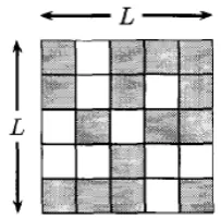
Another way of percolation model is site percolation, which is concerned with whether the grid (called site) is occupied, rather than the edge of the opening or not. Assuming that each lattice point is occupied independently with probability P, the probability 1 − P is not occupied [5]. If the occupied grid points are adjacent to each other, then they form a cluster. The adjacent judgment rule is consistent with the cellular automaton, which uses the von Neumann (Neumann Von.) model, which is the upper, lower, left and right adjacent four cells of a cell [6]. In Figure 3, a total of 5 clusters, from top to bottom, from left to right, the 5 cluster area were 2, 7, 1, 4, 1 units. The area of the largest clusters was 7.

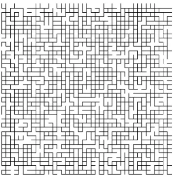
In this paper, we use a stochastic method to generate an example of site percolation.

Figure 1. Bond percolation, P = 0.25.

Figure 3. Example of site percolation.

3. Two Methods of Calculating the Cluster Density

In the following, the small cluster density in the percolation model is calculated by the exact method and the numerical method. Here only consider the area of 1, 2, 3 of small clusters.

3.1. Cluster Number Density-Excat Method

According to paper [5], the exact expression for the number densities of small clusters in two dimensional per-colation model is Formula (1).

( )

( )

t 1

n s, p g s, t (1 p) p

∞

=

=

∑

In Formula (1), g(s, t) represents the number of all clusters with size s and perimeter t. Even though there is no special relationship between the cluster size s and its perimeter t, as it is not on the Bethe lattice, we can enumerate g(s, t) by hand for small cluster sizes. Through this method, we get the following formula.

( )

( )

( )

( )

( )

8 7 3

10 9 8 4

12 11 10 9 8 5

n 1, p (1 p) p

n 2, p 2(1 p) p

n 3, p 2(1 p) 4(1 p) p

n 4, p 2(1 p) 8(1 p) 9(1 p) p

n 5, p 2(1 p) 12(1 p) 28(1 p) 20(1 p) (1 p) p

= − = −   =_ − + − _   =_ − + − + − _   =_ − + − + − + − + − _ (2)

These are the exact expression of the number density of clusters up to size five. Table 1 lists all patterns for small clusters with the area four or smaller. Figure 4 shows three of them: S = 2, S = 3 & t = 7, S = 4 & t = 8. We found that there are three patterns when S = 4, t = 8.

Then we calculate the density of small clusters following Formula (2). The results are shown in Figure 5. The horizontal value is P and the vertical value is density. From Figure 5, we can get the conclusion that the density of all three kinds of small clusters reaches the highest value between P = 0.1 and 0.2.

3.2. Cluster Number Density-Numerical Method

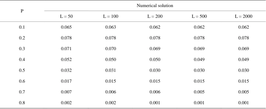
Now we will use the numerical method to calculate the density of clusters. Taking S = 1 as an example, the cal-culation method is as follows: generate the percolation model taking different P (conduction ratio) and different L (the length of the side), then calculate the number of S = 1 using the von Neumann (Neumann Von.) type neighbor, then get the density by using the number divided by the area. In the real calculation, we take combina-tions of P = 0.1, 0.2, 0.3, 0.4, 0.5, 0.6, 0.7, 0.8, L = 50, 100, 200, 500, 2000 and calculate 20 times for each combination and get the average. Table 2 shows the data of one example.

From the data in Table 2, as L is increasing, the densities for each P are almost the same. We use the same method for S = 1, 2, 3.

4. Discussion

Figure 4. Graphs of the three patterns.

Figure 5. Density of small clusters.

Table 1. Patterns and g(s, t) for small clusters, s ≤ 4.

S t Number of patterns g(s, t)

1 4 1 1

2 6 1 2

3 7 1 4

3 8 1 2

4 8 3 9

4 9 1 8

4 10 1 2

Table 2. The density in models of different P and L (S = 1).

P

Numerical solution

L = 50 L = 100 L = 200 L = 500 L = 2000

0.1 0.065 0.063 0.062 0.062 0.062

0.2 0.078 0.078 0.078 0.078 0.078

0.3 0.071 0.070 0.069 0.069 0.069

0.4 0.052 0.050 0.050 0.049 0.049

0.5 0.032 0.031 0.030 0.030 0.030

0.6 0.017 0.015 0.015 0.015 0.015

0.7 0.007 0.006 0.006 0.005 0.005

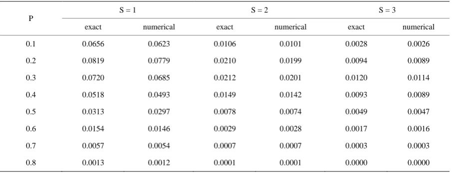
According to Table 3, the results of these two methods are close. Now we discuss the advantages and disad-vantages of each method.

The advantage of exact method is that the calculation is really fast while the formulas are complex, especially when S gets larger. In fact, we now only have the foemula for clusters up to size 40. We cannot construct a theory of percolation based onclusters up to size s = 40-we must consider clusters of all sizes. Therefore, we must recognize that we cannot work out the exact solutions of the cluster number density for all cluster sizes. Since exact solutions are not available for large cluster sizes, we resort to the numerical approach to obtain the general form of the cluster number density n(s,p) for any s and p.

The disadvantage of numerical method is that it is relatively slow, especially when L gets larger. Figure 6 show the relationship between the cluster size and the time taken. The horizontal value is L = 500, 1000, 2000, 5000. The vertical value shows the time in seconds. The time is measured for calculating 20 times. Our test en-vironment is Intel Core i5CPU @1.70 Ghz 2.40 Ghz, 8 GRAM, Windows 7 64bits, python3.5.

In Figure 6, the abscissa said the side length of the square model, the vertical axis represents the calculation time. From Figure 6, the time taken is a most of square (2.0151) relationship of L. The correlation coefficient is 0.99. It takes about 543 seconds to calculate the cluster number density (S = 1) when L = 5000. However, the programs are the same, we barely changed the programs even if S gets large, so it is convenient.

5. Conclusions

Firstly, this paper introduces the percolation model, the bond percolation model and the site percolation model, and introduces how to construct the percolation model.

Figure 6. The relationship between the model size and the time taken.

Table 3. The comparison of the results of exact and numerical method (S = 1, 2, 3).

P

S = 1 S = 2 S = 3

exact numerical exact numerical exact numerical

0.1 0.0656 0.0623 0.0106 0.0101 0.0028 0.0026

0.2 0.0819 0.0779 0.0210 0.0199 0.0094 0.0089

0.3 0.0720 0.0685 0.0212 0.0201 0.0120 0.0114

0.4 0.0518 0.0493 0.0149 0.0142 0.0093 0.0089

0.5 0.0313 0.0297 0.0078 0.0074 0.0049 0.0047

0.6 0.0154 0.0146 0.0029 0.0028 0.0017 0.0016

0.7 0.0057 0.0054 0.0007 0.0007 0.0003 0.0003

On this basis, the density of small clusters (2, 3, 1) in the percolation model are calculated respectively by us-ing the exact method and numerical method, and the results of the two methods are very close.

We find that the cluster density of all three kinds of small clusters reaches the highest value when the occupa-tion probability is between 0.1 and 0.2.

Finally, we discuss the advantages and disadvantages of the two methods, and the advantages of the exact method is that the calculation speed is fast, but the disadvantage is that the formula of the input is very cumber-some, especially when the S is very large.

The disadvantage of the numerical method is that the computation speed is slow, especially when the L is large. However, the numerical method has the advantage of code general, when S is very large, we almost do not have to rewrite the code, it is very convenient. It is very difficult to get the analytical formula for the exact me-thod, such as S = 50, which is very difficult to get the analytical formula for the exact method.

References

[1] Broadbent, S. and Hammersley, J. (1957) Percolation Processes I. Crystals and Mazes. Proceedings of the Cambridge Philosophical Society, 53, 629-641.

[2] Newman, C.M. and Schulmang, L.S. (1981) Number and Density of Percolating Clusters. J. Phys. A: Math. Gen., 14, 1735-1743.

[3] Hongler, C. and Smirnov, S. (2009) Critical Percolation: The Expected Number of Clusters in a Rectangle. Probability Theory & Related Fields, 151, 735-756.

[4] Xiao, L.Q. and Zhou, S.P. (2014) Stochastic Simulation Method and Its Application. Peking University Press, 246-249. [5] Christensen, K. and Moloney, N.R. (2005) Complexity and Criticality. 35-36.

[6] Burks, A.W. Essay on Cellular Automata. University of Illinois Press, Urbana.

Yoshio Yuge, H. (1978) Renormalization-Group Approach for Critical Percolation Behavior in Two Dimesions. Phys Rev (B), 18, 1514-1517.

Submit or recommend next manuscript to SCIRP and we will provide best service for you:

Accepting pre-submission inquiries through Email, Facebook, LinkedIn, Twitter, etc. A wide selection of journals (inclusive of 9 subjects, more than 200 journals) Providing 24-hour high-quality service

User-friendly online submission system Fair and swift peer-review system

Efficient typesetting and proofreading procedure

Display of the result of downloads and visits, as well as the number of cited articles Maximum dissemination of your research work