On Dimension Reduction using Supervised Distance
Preserving Projection for Face Recognition
S.
Jahan
Department of Mathematics, University of Dhaka, Bangladesh
Copyright c2018 by authors, all rights reserved. Authors agree that this article remains permanently open access under the terms of the Creative Commons Attribution License 4.0 International License
Abstract
Personal identication or verification is a very com-mon requirement in modern society specially to access re-stricted area or resources. Biometric identification specially faces identification or recognition in a controlled or an un-controlled scenario has become one of the most important and challenging area of research. Images often are represented as high-dimensional vectors or arrays. Operating directly on these vectors would lead to high computational costs and storage demands. Also working directly with raw data is difficult, challenging or even impossible sometimes. Dimensionality duction has become a necessity for p processing data, re-presentation and classification. It aims to represent data in a low-dimensional space that captures the intrinsic nature of the data.In this article we have applied a Supervised distance preser-ving projection (SDPP) technique, Semidefinite Least Square SDPP (SLS-SDPP), we have proposed recently to reduce the dimension of face image data. Numerical experiments conducted on very well-known face image data sets both on gallery images and blurred images of various level demonstrate that the performance of SLS-SDPP is promising in comparison to two leading approach Eigenface and Fisherface.
Keywords
Supervised Distance Preserving Projection, Semidefinite Programming, Alternating Direction Method of Multipliers.1
Introduction
Personal identication or verification is a very common re-quirement in modern society specially to access restricted area or resources, to travel abroad etc. Biometric identification sy-stems are now being used almost everywhere as it is more se-cure and user-friendly. So this area is getting more focus from researchers. The most common biometric techniques are auto-mated recognition of fingerprints, faces, iris, retina, hand print and voice. Also video surveillance system has become a po-pular systems in terms of security. So, face identification or
recognition in a controlled or an uncontrolled scenario has be-come one of the most important and challenging area of rese-arch.
A general face recognition problem can be stated as follows:
Given a set of face images labeled with the persons identity (the training set) and an unlabeled set of face images from the same group of people (the test set). The aim is toidentify each per-son in the test set.
In a face recognition problem, an image is considered as a high dimensional vector where each of the coordinates corre-sponds to a pixel value in the sample image. Operating di-rectly on these vectors would lead to high computational costs and storage demands. Also working directly with raw data is difficult, challenging or even impossible sometimes. Dimen-sionality reduction has become a necessity for pre- processing data, representation and classification.
In recent years, Deep Learning (DL) method has been success-fully used for image dimensional reduction and recogni-tion. Deep Learning is a machine learning that adapts neu-ral network architecture and consists of multi-layer perceptron (MLP). The method works well on a wide range of large da-tasets. Deep learning uses the Convolution Neural Network (CNN). One of the advantages of using CNN is that compu-ting is so detailed that the rate of error is likely small. But DL is very helpful in solving problems that have a large amount of data which leads to the training process to be long enough and so computing is very complex, directly proportional to the complexity of the problems encountered [29].
This article is concerned with the application of our propo-sed model SLS-SDPP
(P)maxhΨ, Xi − 1
nkUk
2
s.t.AX−U =b
X ∈Sm +
two leading methods Eigenface [31] and Fisherface [2] both in controlled and uncontrolled scenario. Numerical experiments are conducted on three very well-known data set Human face data, Yale and ORL. For the classification taskk-NN algorithm is applied on the reduced dimensional vectors.
2
Previous Studies
Many face recognition techniques have been developed over the past few decades. A complete survey can be found in [9, 33]. Though some of these systems successfully complete the job in constrained scenarios, the general task of face recognition still poses a number of challenges.
Among different techniques, one of the well-established and successful method is appearance-based method [22, 31, 27] which uses the high dimensional (n×m;eg.64×64 = 4096) vector as input to a classifier. Though this technique works well for classifying frontal views of faces they are highly sen-sitive to pose variation. Another alternative to the appearance based approaches is component base technique which matches templates of different facial regions (both eyes, nose, mouth) independently. Some efficient appearance based (also known as global approach) and component base techniques are propo-sed in [21, 15, 19]. Despite the success of these techniques, working with high dimensional (eg. 4096) dataset lead to high computational and storage demands. A possible solution for re-ducing this storage amount and speeding-up the computations is to use feature extraction methods. Previous works have de-monstrated that dimensionality reduction provides an efficient way to detect intrinsic structures of data as well as to extract a reduced number of variables that capture the most relevant features of the high-dimensional data. In the last decades dif-ferent linear and nonlinear dimension reduction methods such as, principal component analysis (PCA) and an its nonlinear variants (KPCA) [16, 17, 2], local linear embedding (LLE), Curvilinear component analysis (CCA) are being used by se-veral authors to reduce the dimension of face image vectors.
Turk and Pentland introduce the Eigenface method for face recognition [31]. A well-known method Fisher face proposed by Belhumeur et al. [2] uses PCA for dimension reduction step and LDA for the classification. Zhuang et al [35] proposed to use Inverse Fishers discriminant criteria (IFFace) as Fisher Face method might fail for some dataset. Some other well-known subspace learning algorithms are Locality Preserving Projection (LPP) [14], Neighborhood Preserving Embedding (NPE) [13], Local Discriminant Embedding (LDE) [8]. Cai et al [11] proposed regularized subspace learning model using a Laplacian penalty to constrain the coefficients to be spatially smooth. Kukharev and Forczma´nski used few variants of Karhunen-Loeve Transform (KLT) and Linear Discriminant Analysis (LDA) [20]. Manifold learning techniques such as ISOMAP [30], LLE [25] and Laplacian Eigenmap [3] consider nonlinear dimensionality reduction by investigating the local geometry of data. These techniques are good for representation, but only concern with the training data.
Most of the above dimensionality reduction techniques preserves the local structure or focused on the global structure. So building a method that preserves local structure as well as maximizes the global variance can be more reliable for a classification problem.
In the next section we have briefly discussed our proposed method SLS-SDPP and the method is applied to reduce the dimension of face image data in the following section. Nu-merical experiments conducted on very well-known data set Yale and ORL showed remarkable performance of SLS-SDPP in comparison to two leading methods Eigenface [31] and Fisherface [2] both in controlled and uncontrolled scenario.
3
Supervised Distance Preserving
Pro-jection (SDPP)
The Supervised Distance Preserving Projection (SDPP) is a dimensionality reduction method that minimizes the differen-ces between distandifferen-ces among projected co-variates and distan-ces among responses locally. That means, the local geome-trical structure of the low dimensional subspace preserves the geometrical characteristics of the response space. It also pre-serves the continuity of the response space.
The idea of SDPP is to represent high dimensional (m- dimen-sional )data{x1, x2, ...., xn} in a lower dimensional spaceZ with dimensionalityr << m
The form of data representation in<r, denoted asf, is as-sumed to be a linear function of the feature vector xin the original input space, defined by
f(x) =WTx, ∀x∈ <m (1) where the transformation matrixW ∈ <r×m. Therefore the objective is to minimize F(W) = 1
n P
ij(d 2
ij(W)−δij2)2, whered(,)andδ(,)are distance functions inZ andY space respectively.
In [34] Zhu et al. first proposed the methodology. To pre-serve the local structure of the data Zhu has incorporated a neighborhood graph Gij in the objective function defined as follows:
Gij=
1 ifi∼j(k−N N neighbor) 0 otherwise,
The schematic illustration of neighborhood selection of SDPP is given in APPENDIX A. Thus the objective of SDPP is to minimize
F(W) = 1
n
X
ij
Gij(d2ij(W)−δ 2 ij)
2 (2)
4
SDPP as Semidefinite Least Square
(SLS-SDPP)
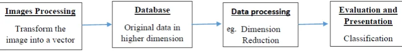
Figure 1:Basic steps of Face recognition procedure
stay together and therefore preserves the global structure in the projected space. The objective of our model thus becomes
max n X
i=1
kzik2−
ν n
X
ij
Gij(d2ij(W)−δij2)2 (3)
A more compact form of this model is obtained after some al-gebraic manipulations reported in Appendix B: Thus we have the Matrix form of SLS-SDPP
(P)maxhΨ, Xi − 1
nkUk
2
s.t.AX−U =b
X ∈Sm +
Note that a similar type problem is previously studied by Ji-ang et al in [18] where they developed a Partial Proximal Point algorithm to solve the problem. In the next section we will study a two block Alternating Direction Method of Multiplier to solve SLS-SDPP problem (P).
5
ADMM for SLS-SDPP
Alternating Direction Method of Multipliers [5] is a very ef-ficient and important algorithm that solves convex optimization problem by breaking it into smaller and easier optimizations problems. Due to its simplicity and efficiency it has recently found many applications in several areas like imaging science, signal processing, machine learning etc.
We hereby developed a two block ADMM algorithm for our SLS-SDPP problem. Derivation of the augmented Lagrange functionLσ(z, S;X)used in the algorithm is given in APPEN-DIX C.
Algorithm 1. Alternating Direction Method of Mul-tipliers
Given parametersτ∈(0,∞).
(S.0) Chooseσ0>0,S0∈S+m,
X0 = W0W0T ∈ S+m. Set z0 = (n2I + σAA∗)−1 b−AX0+σA(−Ψ−S0)
. Letk= 0.
(S.1) UpdateSk
by
Sk+1= arg minLσk(z
k , S;Xk) = ΠSm
+
−Ψ−A∗ zk−Xk
σk
(S.2) Updatezkby
zk+1= arg minLσk(z, S
k+1
;Xk)
=(n2I+σAA∗)−1(b−AXk+σA(−Ψ−Sk+1))
(S.3) UpdateXkby
Xk+1= arg minL σk(z
k+1, Sk+1;X)
=Xk+τ σk(A∗zk+1+Sk+1+ Ψ)
(S.4) Updateσkby
σk+1=ρσkor σk+1=σk (4)
Note that
• In (S.1), the projectionΠSn
+(X1)of a given matrixX1∈ SnontoSn
+is the optimal solution of the problem
min 1
2kY −X1k 2
s.t. Y ∈Sn +
• In (S.2), to updatezwe need to solve linear systems in-volving the operatorAA∗. The computation ofAA∗ and its (sparse) Cholesky factorization, which only needs to be done once, can be done at a moderate cost.
In [28] Sun et al. discussed a similar type 3-block semi-proximal ADMM for conic optimization problem.
The convergence of algorithm 1 for solving problem (D) fol-lows from the theorem established in [28] which is discussed in APPENDIX. .
6
Problem Formulation
Given a set of N sample images {x1, x2, . . . , xN} in an n-dimensional image space and assuming that each image belongs to one of thelclassesC1, C2, ...., Cl, consider a linear transformation z = WTx from the original n-dimensional image space into an m-dimensional feature space, where
m < nand whereW ∈ <n×mis a matrix with orthonormal columns. HereWT is the transformation matrix from higher dimensional image space to the lower dimensional space. Different techniques have been used by several researchers to determine this transformation matrix W. Here we have briefly discussed the idea of two leading methods Eigenface and Fisherface.
6.1
Eigenface
Eigenface method uses Principal Component Analysis (PCA) to reduce the dimension of the image space by maxi-mizing the total scatter of all projected samples. If the total variance matrixSis defined by:S=PNi=1(xi−µ)(xi−µ)T whereµ∈ <nis the mean image of all samples andS ∈ <n×n, then the basic idea of Eigenface method is to determine the transformation matrixW in such a way that the determinant of the total scatter matrixWTSW of the projected sample is maximized. Thus the objective function of Eigenface method is
max W∈<n×m |W
TSW| (5)
The m columns of the optimum matrix W is the set of n
dimensional eigenvectors corresponding tomlargest eigenva-lues of the matrixS. Each of this eigenvectors having the same dimension as the original images, referred to as Eigenpictures or Eigenfaces.
Note that the Eigenface method doesn’t use the class infor-mation of the images to determine the projection matrix.
6.2
Fisherface
Since the main intention of face recognition problem is to identify the classes of test images, so using the class informa-tion of the training images in determining the transformainforma-tion matrixW may increase the classification rate. Based on this idea Belhumeur proposed the Fisherface method in [2] which uses Fishers Linear Discriminant (FLD). This method selects
W in in such a way that the ratio of the between-class scatter and the within class scatter is maximized.LetSbbe the between class scatter matrix defined bySb =Pli=1Ni(µi−µ)(µi−µ)T andSwbe the within class scatter matrix defined by
Sw = Pl
i=1(xi −µi)(xi−µi)T. µi is the mean of sample images of classCiandNiis the number of images in classXi. IfSwis nonsingular, the optimal projectionWoptis chosen as the matrix with orthonormal columns which maximizes the ra-tio of the determinant of the between-class scatter matrix of the projected samples to the determinant of the within-class scatter
matrix of the projected samples. That is,
Wopt=argmax W
|WTS bW|
|WTS wW|
Themcolumnsw1, w2, . . . , wmof optimumW are the ge-neralized eigenvectors corresponding to themlargest genera-lized eigenvaluesλiofSbandSw. That is,Sbwi =λiSwwi.
Note thatm≤l−1, wherelis the number of classes, since the maximum number of nonzero generalized eigenvalues is
l−1[2].
In the face recognition problem, one is confronted with the dif-ficulty that the within-class scatter matrixSw ∈ <n×n is al-ways singular. This stems from the fact that the rank ofSwis at mostN−l, and, in general, the number of images in the le-arning setN is much smaller than the number of pixels in each image n. This means that it is possible to choose the matrixW
such that the within-class scatter of the projected samples can be made exactly zero. In order to overcome the complication of a singularSw, Belhumeur proposed the following alterna-tive methodology in [2].
Fisherface method uses two steps to determine the optimum transformation matrixWopt. First step is to reduce the dimen-sionnof the original image space toN −lusing PCA so that the resulting within-class scatter matrixSwis nonsingular. The second step is to apply the Fishers Linear Discriminant (FLD) (which uses the class information of the training images) on the transformed data to reduce the dimensionN−ltom. Thus Fisherface method aims to determine the matrixWoptT =
WT F LDW
T
P CAfrom the following two steps: Step 1: WP CA= arg maxW∈<n×(N−l)|WTSW|
Step 2: WF LD = arg maxW∈<(N−l)×m| WTWT
P CASbWP CAW| |WTWT
P CASwWP CAW|
In step 1,Sis the variance matrix of total sample and theN−l
columns of the optimum matrixWP CAis the eigenvectors cor-responding toN−llargest eigenvalues of the matrixS. In step 2,Sb, and Sw are the between class and withn class scatter matrix defined earlier.
In Fisherface method though PCA at the first step is used to avoid the nonsingularity of the within class scatter matrixSw, this PCA step doesn’t guarantee the nonsingularity of the trans-formed covariance matrix [35]. On the other hand, a dra-wback of Eigenface method is that the maximization of to-tal variance not only maximizes the between class scatter but also the within class scatter which leads to lower classification rate.(Verified by numerical experiments.)
In view of these limitations, we propose to use our model SLS-SDPP that maximizes the variance of the total sample and pre-serves the distances of local points by minimizes the differen-ces between distandifferen-ces among projected co-variates and distan-ces among responses locally.
6.3
SLS-SDPP
Figure 2:Overview of Face recognition method using dimension reduction.
At the same time SLS-SDPP maximizes the variance of total sample that prevents the different class of images to be pro-jected very close, therefore preserves the global structure. Thus the objective of our proposed approach SLS-SDPP is
maxW∈<n×m n X
i=1
kWTxik2−
ν n
X
ij
Gij(d2ij(W)−δ 2 ij)
2
Here we have applied our proposed algorithm Alg. 1 to determine the projection matrixW. NN- rule is further applied to identify the classes of the images.
An overview of face recognition methods using dimension re-duction is shown in Fig. 2. All of the three methods discussed above follow these basic steps to identify the class of the test images.
7
Recognition from gallery image:
In this section we will apply Eigenface, Fisherface and SLS-SDPP on two very well-known face data set Yale and ORL. Yale data base is mainly generated by Computer Vision Laboratory in the Computer Science and Engineering Department at University of California San Diego and the ORL database is constructed at AT&T laboratories Cambridge.
Yale Face Database
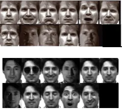
Yale face database contains 165 gray scale images of 15 indi-viduals. There are 11 images per subject with size243×320, with different facial expression or configuration: one normal image under ambient lighting, two with or without glasses, three images taken with different point light sources (centre, left, right), and five different facial expressions(happy, sad, sleepy, surprised and wink). Fig. 3 depicts total 22 samples of two individuals (11 samples of each individual) of Yale face data .
Olivetti Research Laboratory ORL database
The ORL contains 10 different images of each of the 40 dis-tinct subjects of size92×112. The images were taken at diffe-rent times, varying the lighting, facial expressions (open / clo-sed eyes, smiling / not smiling) and facial details (glasses / no
Figure 3:Illustration of face images with different lighting condition and fa-cial expression of two individuals from Yale database.
glasses). All the images were taken against a dark homogene-ous background with the subjects in an upright, frontal position (with tolerance for some side movement). Some examples of ORL faces with different facial expressions and lighting con-ditions are given in Fig. 6.
7.1
Pre-Processing Step:
In our experiments we used the
pro-cessed Yale and ORL data obtained from
http://www.cad.zju.edu.cn/home/dengcai/Data
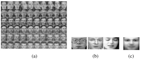
/FaceData.html processed by Cai et al [11]. All the face images are manually aligned and cropped. A sample of cropped images and the mean of all the cropped faces are shown in Fig. 4 and Fig. 6. The size of each cropped image is64×64pixels, with 256 gray levels per pixel. Thus each image is represented as a 4096-dimensional vector. Both the datasets are preprocessed by mean centering and normalized to unit variance.
For each of the data sets a random subset with p (= 2,3,4,5,6,7,8) images per individual was taken with labels to form the training set and the rest of the images were consi-dered to form the testing set. For example, for Yale data set, each of 15 individuals have 11 images. So the training set with
[image:5.595.365.490.284.397.2]Table 1:Average recognition rate of Yale test sample achieved by SLS-SDPP, Fisherface and Eigenface methods along different number of training points.
T Rp SLS-SDPP Fisherface Eigenface
Recognition Rate (mean±std)
[image:6.595.116.480.225.317.2]T R2 0.6529±0.0561 0.3421±0.0382 0.5040±0.0238 T R3 0.7167±0.0460 0.7422±0.0362 0.5582±0.0426 T R4 0.7429±0.0492 0.4617±0.2254 0.5901±0.0307 T R5 0.7444±0.0311 0.7889±0.0213 0.6127±0.0346 T R6 0.7867±0.0401 0.8763±0.0353 0.6213±0.0410 T R7 0.8233±0.0324 0.8897±0.0408 0.6233±0.0426 T R8 0.9189±0.0353 0.6841±0.2856 0.6409±0.0659
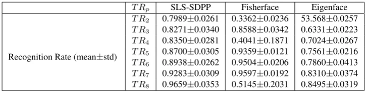
Table 2:Average recognition rate of ORL test sample achieved by SLS-SDPP, Fisherface and Eigenface methods along different number of training points.
T Rp SLS-SDPP Fisherface Eigenface
Recognition Rate (mean±std)
T R2 0.7989±0.0261 0.3362±0.0236 53.568±0.0257 T R3 0.8271±0.0340 0.8588±0.0342 0.6331±0.0223 T R4 0.8350±0.0281 0.4041±0.1871 0.7024±0.0267 T R5 0.8700±0.0305 0.9359±0.0121 0.7561±0.0216 T R6 0.8938±0.0262 0.9504±0.0206 0.7860±0.0413 T R7 0.9283±0.0309 0.9597±0.0192 0.8310±0.0374 T R8 0.9659±0.0353 0.5145±0.2031 0.8495±0.0319
are 50 randomly splits into training and testing images. For the classification task, we used 1-Nearest Neighbor rule. The re-cognition rate is calculated as the ratio of number of successful recognition and the total number of test samples. In the same manner, the error rate is calculated as the ratio of number of failure in recognition to the total number of test samples.
7.2
Experimental results:
The projection quality usually varies with the number of dimensions. So for each of the dataset first we have determined the dimension of the projected space. For Fisheface method the dimension is chosen to be (No. of classes-1)[2]. For Eigenface method, first D eigenvectors are chosen, where (D=Number of training samples)[2]. For SLS-SDPP, we choose the dimension of projected space by observing the performance of the method at different dimension. Fig. 5(a) represents the recognition rate in identifying the test faces of Yale dataset with different training samples (T R6, T R7, T R8) along different dimension which suggested us to project the Yale data set in 9 dimensional space. For ORL dataset we choose 41 relevant features to predict the class of test samples as SLS-SDPP obtains best result atD = 41 for ORL which can be verified from Fig. 7(a). The parameter (neighborhood)
k is chosen to be between 2-6 using cross validation in the training samples of each of the data set.
A 2D projection of the Yale data base and ORL database obtained by SLS-SDPP are depicted in figure Fig. 5(b) and Fig. 7(b). Sample of the test images of both datasets are superimposed on the respective 2D plots which shows that images of same individuals are clustered and therefore proves the preservation of local structure of the data.
The average recognition accuracy of all the three algorithms along different number of training images of Yale and ORL databases are presented in Fig. 8 which is also reported on the
Table 1 and 2 respectively. For eachT Rp, wherepis the num-ber of training image, we took average of the results over 50 random splits and reported the mean as well as the standard deviation.
Table 1 shows that for SLS-SDPP, the average recognition rate increases from66%to92%with the increase in number of training images from 2 to 8. Eigenface method also fol-lows the same pattern but obtains much lower recognition rate in comparison to SLS-SDPP. Moreover the small standard de-viation indicates the stability of our algorithm as well as Ei-genface regarding the random splitting. However Fisherface method shows a different pattern. It gives best performance for training samples with 7 images of each individual. Fig. 8(a) illustrates that the recognition rate of Fisherface drops drasti-cally when the number of training images per class is 8 and 4. Also its performance is very much unstable in this cases which can be observed from the large values of std,23%forp = 4 and29% forp = 8) recognition rate in comparison to other two methods which can also be observed from Fig. 8(a) . Similar to Yale face database, for ORL data set our method out-performs Eigenface method and Fisher face method (in some case). The improvement of recognition rate of the test ima-ges in our algorithm for ORL data set is from79% to 96% with the increase of number of training samples. Though for both Yale and ORL dataset Fisherafce gives better recognition rate than our method for some values ofp, its performance is unstable whereas our method shows a consistent performance throughout the experiment which is beneficial for practical ap-plications with any training sample size.
8
Recognition from Blurred image:
condi-(a) (b) (c) (d) Mean Yale face
Figure 4:(a)-(c) Sample of original and cropped face images from Yale database. (d) Mean face of Yale database
[image:7.595.151.446.192.324.2](a) Recognition rate along different dimension (b) Test images of yale database superimpo-sed on corresponding data point (red circle)
Figure 5:(a) Recognition rate of test sample of Yale face image along different dimension. The experiment is carried out by SLS-SDPP for different number of training samples TRp( p indicates the number of different images of each individual). Maximum recognition rate achieves at dimensionD = 9. (b) 2D projection of Yale test faces and a sample of them superimposed on corresponding data points (red circle). Images of same class are seen to be projected closely.
(a) (b) (c)
Figure 6:(a)-(b) Illustration of facial expression variation of some in-dividuals from ORL database, (c) Sample of cropped ORL faces. (d) Mean face of ORL database
tions, performance of most face identification algorithms drop drastically. Various methods have been proposed to deal with the recognition of blurry images [12, 26, 1]. In this section we have conducted numerical experiments on various level of artificially blurred images using the three methods SLS-SDPP, Eigenface and Fisheface to demonstrate their behavior in re-cognizing blur faces.
8.1
Pre-processing step:
To test the performance of the algorithms in uncontrolled scenery, we have artificially generated set of blurred images from Yale and ORL datasets. For the degradation step, Gaus-sian filter available in MATLAB library is applied on the ori-ginal images. The set of blurred images shown in Fig. 9 corre-sponds to the standard deviationsσ= 2,4,6and8respectively withmasksize= 1.5∗σ. The training set is degraded to the same blur level of the test set to do the matching.
8.2
Experimental results:
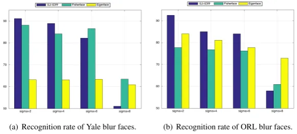
The recognition rate of test samples for Yale and ORL data set along different level of blur images are depicted in Fig. 10. The bar diagrams illustrate that performance of SLS-SDPP is consistent along various blur level. For Yale dataset the re-cognition rate varies approximately from92%to88%and for ORL data it varies from93% to84% as the standard devia-tion varies from 2 to 6. Note that for each of the datasets, the prediction rate drops suddenly for SLS-SDPP and Fisherface when standard deviation sigma = 8. For Yale face data-set, though the recognition rate of Eigenface method remained much lower than other two methods through out the experi-ment, it shows almost the same performance for any level of blur images which is beneficial for face recognition problems with much blur effect. Same behaviour of Eigenface method can also be observed for ORL database. However, for both of the data set the SLS-SDPP outperforms other two methods in most of the cases.
9
Conclusion
[image:7.595.53.279.391.487.2](a) (b)
[image:8.595.113.485.290.440.2]Figure 7:Figure shows (a) Success rate of SLS-SDPP in predicting of ORL test images along different dimension.The experiment is carried out for different number of training samples. Highest recognition rate achieved at dimension D=41. (b) 2D projection of ORL test faces and a sample of them superimposed on corresponding data points (red circle). Images of same class are seen to be projected closely.
Figure 8:Average recognition rate of faces along different number of training samples, left figure for Yale dataset and right one for ORL dataset. Though Fisherface gives better recognition rate than our method in some cases , its performance is much unstable whereas SLS-SDPP shows a consistent performance throughout the experiment.
Figure 9:Example of images artificially blurred with standard deviation (σ=1(origin),2,3,4,5 respectively) of Gaussian filter. (a) Yale face (b) ORL face.
(a) Recognition rate of Yale blur faces. (b) Recognition rate of ORL blur faces.
[image:8.595.132.459.501.565.2] [image:8.595.150.442.606.738.2]become a necessity for preprocessing data for representation and classification.
In this work we have addressed application of our proposed distance preserving dimension reduction method SLS-SDPP on gallery images and blurred images of various level. Numerical experiments on both gallery and probe images demonstrate that the performance of our algorithm is promi-sing in comparison to two leading approach Eigenface and Fisherface. Eigenface method obtains much lower recognition rate in comparison to SLS-SDPP. Though Fisherface gives better recognition rate than our method in some cases , its performance is much unstable whereas our method shows a consistent performance throughout the experiment which is beneficial for practical applications with any training sample size.
For testing the blur images we assumed that we have the blur degree of the testing image which we used to degrade the training images. In real problems with test images of unknown blur level, several methods [12, 23, 24] exist to infer the blur degree of the images which can be used to degrade the training set or deblur the testing set. A detailed descriptive work on this area is beyond the scope of this research work and is planned to be considered in future. Also further research will focus on improving the transformation learning matrix to apply on images with other uncontrolled scenario mentioned above as well as other image recognition problems such as finger print, digit, signature etc.
Appendices
A
SDPP
Suppose we havendata points{x1, x2, ...., xn}, xi ∈ <m and their responses{y1, y2, ..., yn}.
The method seeks for the transformation matrixW that mi-nimizes
F(W) = 1
n
n X
i=1 X
xj∈N(xi)
(d2ij(W)−δ2ij)2
whereN(xi) denotes a neighborhood of xi, Euclidean me-tric is used to characterized the pairwise distances; that is
d2
ij(W) =kzi−zjk2andδijtakes the following form:
δij = 0
ifi∼j(xiand xjbelongs to same class) 1 otherwise,
SDPP that has to be set beforehand or tuned from data. In [34] the value of k selected by a continuity measure.
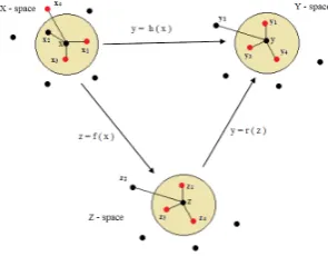
The schematic illustration of SDPP [34] is given in Fig. 11. For a point x in input space, consider three nearest neighbor
N(x) ={x1, x2, x3}. Suppose in output space the neighbor-hood ofyis{y1, y3, y4}ie.y2is outside of the neighborhood ofy. SDPP seeks for the transformation matrixW for which
z2=f(x2)is moved outside the neighborhood in theZ-space whilez4 is moved inside to match the local geometry in the
Y-space as shown in Fig. 11 and Fig. 12.
B
Reformulation as SLS-SDPP
To reformulate problem 2 as Semidefinite Matrix least Squa-res with linear equality constraints. First we rewrite the square of the pairwise distance in theZ-space as
d2ij(W) =kWT(xi−xj)k2=h(xi−xj)(xi−xj)T, W WTi
LetΦij = (xi −xj)(xi−xj)andX = W WT. Then the objective functionF(W)in 2 takes the form
f(W) = 1
n
X
i,j
Gij(hΦij, Xi −δ2ij)
2 (6)
whereGijis defined before in section 3. HereG∈ <n×n, X∈
<m×m,Φ
ij ∈ <m×m,(i, j)∈ξ
Letuij =hΦij, Xi −δij2. Then, the optimization model that of SDPP can be written as
min f(W) = 1
n
X
i,j
GijkUk2 (7)
such thathΦij, xi −uij =δij2,(i, j)∈ξ.
SupposePni=1xi = 0 i.e{xi}ni=1 is already centralized. Then zi = WTxi, f or i = 1,2, ..., n is also centralized. We incorporate the total variancePni=1kzik2to the objective function 7 where
= n X
i=1
kWTxik2= n X
i=1
hxixTi , W W T
i= n X
i=1
hΨii, W WTi.
DenotingX =W WT, The optimization model is reformula-ted as follows:
maxh
n X
i=1
Ψii, Xi −
ν n
X
i,j
GijkUk2
s.t.hΦij, Xi −uij =δ2ij
X 0
whereν >0,(i, j)∈ξ.
Now denoteΨ = Pni=1Ψii,AX = hΦij, Xi, b = δij2. Let
H = (Gij) > 0where(i, j) ∈ ξ. Herekξk = p = k∗n. ThereforeH ∈ <p.
For a vectorv ∈ <p, we definekvk2 H =
Pp
i=1Hivi2, our ob-jective function can be rewritten as
maxhΨ, Xi −ν
nkAX−bk 2
H=hΨ, Xi − ν nkUk
Figure 11:SDPP: Solid lines indicate connection between neighbors
Figure 12:Preservation scheme of the local geometry by SDPP.
According to the definition ofG= (Gi,j), Hi = 1,∀i. We consider the value of penalty parameterν = 1. Therefore our goal is to find the best value of the matrix X which solves the following Semidefinite Least Square (SLS) problem:
(P)maxhΨ, Xi − 1
nkUk
2
s.t.AX−U =b
X ∈Sm +
C
Augmented
Lagrange
function
L
σ(
z, S
;
X
)
To derive the augmented Lagrange function Lσ(z, S;X), first step is to obtain the dual (D) of the primal problem (P). The next step is to determine the augmented Lagrange function of (D).
Now , Consider the Lagrangian function of the primal pro-blem (P)
L(X,U,z) = hΨ,Xi−1 nkUk
2
F+hz,AX−U−bi+δSm +(X)
= h−b,zi+hA∗z+Ψ,Xi+hz,−Ui−1 nkUk
2
F+δSm+(X).
Therefore the dual function is min
z∈<p
Θ(X, U, z) = max
X∈<m×m,U∈<p L(X, U, z)
.
The dual problem of (P) thus obtained is:
(D)minΘ(z) =−hb, zi+n 4kzk
2
s.t.A∗z+ Ψ +S= 0
S∈Sm +.
For the convergence of 2 block ADMM , we need the fol-lowing assumption which is a simpler version of assumption 1 discussed in section 3.2 of [5]. .
Assumption 2. a) There exists a feasible solutionXˆ ∈Sm + of
problem (P) such thatAX−U =b,Xˆ ∈int(Sm +).
b) There exists a feasible solution{S,ˆ zˆ} ∈Sm
+ × <pof
pro-blem (D) such that
A∗z+ Ψ +S= 0,Sˆ∈int(Sm +).
From convex analysis [6, sec. 5.5.3] [4, Cor. 5.3.6 ] it is known that under assumption 2 the strong duality for (P) and (D) holds and the following Karush-Kuhn-Tucker (KKT) con-ditions has nonempty solution
AX−U =b,A∗z+Ψ+S= 0,hX, Si= 0, X∈Sm +, S∈S
m +. (8) Forσ >0, the augmented Lagrange function for (D) is defined by
Lσ(z,S;X)=−hb,zi+n4kzk
2+hX,A∗z+Ψ+Si+σ 2kA
∗z+Ψ+Sk2 F
=−hb,zi+n 4kzk
2+σ 2kA
∗z+Ψ+S+X
σk
2
F−
kXk2F 2σ ,
where(z, S, X)∈ <p×Sm + ×S+m.
References
[1] Ahonen, T., Rahtu, E., Ojansivu, V. and Heikkil, J. (2008), ‘Re-cognition of blurred faces using local phase quantization’, Pat-tern Recognition InPat-ternational Conference on PatPat-tern Recogni-tion[ICPR], pp. 1–4.
[4] Borwein, J. and Lewis, A.S. (2006), Convex Analysis and Non Linear Optimization : theory and examples,Springer, vol. 3.
[5] Boyd, S., Parikh, N., Chu, E., Peleato, B. and Eckstein, J. (2010), ‘Distributed Optimization and Statistical Learning via the Alter-nating Direction Method of Multipliers’,Machine Learning, vol. 3, no. 1, pp 1–122.
[6] Boyd, S. and Vandenberghe, L. (2004), Convex Optimization,
Cambridge University Press.
[7] Brito, M.R., Chvez, E.L., Quiroz, A.J. and Yukich, J.E. (1997), ‘Connectivity of the mutual k-nearest-neighbor graph in cluste-ring and outlier detection’,Statistics and Probability Letters, vol. 35, no. 1, pp. 33–42.
[8] Chen, H-T., Chang, H-W. and Liu, T-L. (2005), ‘Local discrimi-nant embedding and its variants’,In Proceeding of IEEE Compu-ter Society Conference on CompuCompu-ter Vision and PatCompu-tern Recogni-tion.
[9] Chellapa, R., Wilson, C. and Sirohey, S. (1995), ‘Human and machine recognition of faces: a survey’,Proceedings of the IEEE, vol. 83, no. 5, pp. 705–741.
[10] Coronaa, F., Zhu, Z., Souza Jr, M. Mulasd, A. H. d., Muruf, E., Sassuf, L., Barretob, G. and Baratti, R. (2015), ‘Supervised Distance Preserving Projections: Applications in the quantitative analysis of diesel fuels and light cycle oils from NIR spectra’,
Journal of Process Control, vol. 30 , pp. 10–21.
[11] Cai, D., He, X., Hu, Y., Han, J. and Huang, T. (2007), ‘Learning a Spatially Smooth Subspace for Face Recognition’, Proceeding of IEEE Conference on Computer Vision and Pattern Recognition Machine Learning.
[12] Fichea, C. , Ladreta, P. and Vua, N-S. (2010), ‘Blurred Face Recognition Algorithm Guided by a No-Reference Blur Metric’,
Image Processing: Machine Vision Applications III, France, doi : 10.1117/12.840245.
[13] He, X., Cai, D., Yan, S. and Zhang, H-J. (2005), ‘ Neighbor-hood preserving embedding’, In Proceeding of IEEE Internatio-nal Conference on Computer Vision.
[14] He, X. and Niyogi, P. (2003), ‘Locality preserving projections’,
Advances in Neural Information Processing Systems 16.
[15] Heisele, B., Ho, P. and Poggio, T. (2001), ‘Face Recogni-tion with Support Vector Machines: Global versus Component-based Approach’, In the proceeding of Eighth IEEE In-ternational Conference on Computer Vision, vol. 2, doi: 10.1109/ICCV.2001.937693.
[16] Huang, W. and Yin, H. (2009), ‘Linear and Nonlinear Dimen-sionality Reduction for Face Recognition’16th IEEE Internatio-nal Conference on Image Processing (ICIP), pp. 3337–3340, doi. 10.1109/ICIP.2009.5413898.
[17] Huang, W. and Yin, H. (2012), ‘On Nonlinear Dimensionality Reduction for Face Recognition’, Image and Vision Computing, vol. 30, no. 45, pp. 355–366, doi: 10.1016/j.imavis.2012.03.004.
Publisher: Springer, pp. 133–162.
[19] Jonsson, K., Matas, J., Kittler, J. and Li, Y. (2000), ‘Learning support vectors for face verification and recognition’,In Procee-ding of IEEE International Conference on Automatic Face and Gesture Recognition, pp. 208–213.
[20] Kukharev, G and Forczman´ski, P. (2004), ‘Data dimensionality reduction for face recognition’,Machine Graphics&Vision, vol. 13, pp 99–121.
[21] Lanitis, A., Taylor, C. and Cootes, T. (1997), ‘Automatic inter-pretation and coding of face images using flexible models’,IEEE Transactions on Pattern Analysis and Machine Intelligence, vol. 19, no. 7, pp. 743–756.
[22] Murase, H. and Nayar, S.K. (1995), ‘Visual Learning and Re-cognition of 3-D Objects from Appearance’, International Jour-nal of Computer Vision, vol. 14, 5–24.
[23] Nishiyama, M., Takeshima, H., Shotton,J., Kozakaya, T. and Yamaguchi, O. (2009), ‘Facial deblur inference to improve recognition of blurred faces’, IEEE Conference on Com-puter Vision and Pattern Recognition, pp. 1115–1122, doi: 10.1109/CVPR.2009.5206750.
[24] Nishiyama, M., Hadid, A., Takeshima,H., Shotton, J., Koza-kaya, T. and Yamaguchi, O. (2011), ‘Facial Deblur Inference Using Subspace Analysis for Recognition of Blurred Faces’,
IEEE Transactions on Pattern Analysis and Machine Intelligence, vol. 33, no. 4, pp. 838–845, doi: 10.1109/TPAMI.2010.203.
[25] Roweis, S. and Saul, L. (2000), ‘Nonlinear dimensionality re-duction by locally linear embedding’,Science, vol. 290, no. 5500, pp. 2323–2326.
[26] Stainvas, I. and Intrator, N. (2000), ‘Blurred face recognition via a hybrid network architecture’,Proceedings of 15th International Conference on Pattern Recognition, vol. 2, pp. 805–808.
[27] Sirovitch, L. and Kirby, M. (1987), ‘Low-dimensional pro-cedure for the characterization of human faces’, Journal of the Optical Society of America A, vol. 2, pp. 519–524.
[28] Sun, D., Toh, K.-C. and Yang, L. (2014), ‘A Convergent 3-Block Semi-Proximal Alternating Direction Method of Multipliers for Conic Programming with 4-Type of Constraints’, SIAM Journal on Optimization, vol. 25, no. 2, pp. 882–915.
[29] Setiowati,S., Zulfanahri, Franita, E. L., Ardiyanto, I.(2018), ‘A Review of Optimization Method in Face Recognition: Compa-rison Deep Learning and Non-Deep Learning Methods’, Pro-ceedings of ninth IEEE International Conference on Infor-mation Technology and Electrical Engineering (ICITEE), doi. 10.1109/ICITEED.2017.8250484
[30] Tenenbaum, J., Silva, V. and Langford, J. (2000), ‘A glo-bal geometric framework for nonlinear dimensionality reduction’,
Science, vol.290, no. 5500, pp. 2319–2323.
[32] Venna, J. and Kaski, S. (2007), ‘Comparison of visualization methods for an atlas of gene expression data sets’, Information Visualization, vol. 6, pp. 139–154.
[33] Zhao, W., Chellappa, R., Phillips, P.J., Rosenfeld, A. (2003), ‘Face Recognition: A Literature Survey’, ACM Computing Sur-veys, vol. 35, no. 4, pp. 399–458.
[34] Zhu, Z, Simil¨a, T. and Corona, F. (2013), ‘Supervised Distance Preserving Projection’,Neural Processing Letters, vol. 38, no. 3, pp. 445–463.