Estimating Change Point in Single Server Queues

Estimating Change Point in Single Server Queues

Sibanee Sahu

∗

,

Sarat Kumar Acharya

P. G. Department of Statistics, Sambalpur University, Odisha, India

Copyright c⃝2016 by authors, all rights reserved. Authors agree that this article remains permanently

open access under the terms of the Creative Commons Attribution License 4.0 International License

Abstract

The paper is concerned with the study of change point problem in the inter-arrival time and service time of single server queues. Maximum likelihood estimators of the parameters are derived. A test statistics has been developed and its properties have been studied.

Keywords

Single Server Queue, Maximum Likelihood Estimator, Change Point, Likelihood Ratio

1

Introduction

Statistical inference plays a major role in any use of a queueing models in decision making. Many authors have studied the parameter estimation problem in queueing models. Basawa and Prabhu[4,5] have discussed moment and likelihood estimation of the model parameters for single server queues using various sampling plans. Bhat and Rao [6] have provided an exhaustive survey of results on inference for queueing systems. Basawa and Bhat [2] studied sequential inference for the parameters of a GI/G/1queue. An empirical Bayes approach was used for estimating by Thiruvaiyaru and Basawa [15]. Basawa et al. [3] presented a maximum likelihood method for estimating the parameters of the arrival and service time distribution using only the information on the waiting times of customers inGI/G/1queue with “first come first served” queue disciline. Clarke [10] obtained the maximum likelihood estimates for the arrival and service parameters of anM/M/1 queue. A review of the literature on the subject reveals that so far only single server queues have been considered from an inferential viewpoint. crane and lemoine [14] have applied simulation techniques to the problem of estimating the steady state mean waiting time in a single server queue. Acharya [1] have discussed the rate of convergence of the distribution of the maximum likelihood estimators of the arrival and the service rates in a GI/G/1 model.

Change is a natural phenomenon which occurs in every sphere of works. In statistics we are interested in the statistical analysis of change point detection and estimation.

LetX1, X2, X3, . . . , Xnbe a sequence of independent random variables with probability distribution functionsF1, F2, F3, . . . , Fn,

respectively.

Then, in general, the change point problem is to test the following null hypothesis: H0:F1=F2=. . .=Fn verses the alternative hypothesis

H0:F1=F2=. . .=Fk ̸=Fk+1=. . .=Fn

If the distributionsF1, F2, F3, . . . , Fn belongs to the common parametric familyF(θ), whereθ ∈Rp, then the change

point problem is to test the hypothesis about the population parameterθi, i= 1,2,3, . . . , n,

H0:θ1=θ2=. . .=θn=θ(unknown) verses the alternative hypothesis

H0:θ1=θ2=. . .=θk̸=θk+1=. . .=θn

series models. For relevant references in i.i.d samples and time series models, we refer to Brown, Durbin and Evans[7], Wichern, Miller and Hsu[17], Zacks[18], Krishnaiah and Miao[13] and the references therein.

The problem of estimating change point of the inter-arrival time distribution in the queueing is of great interest. Be-sides maximum likelihood and least square estimates, the Bayesian method is also a very useful technique for estimating parameters. Chernoff and Zacks [8] has studied the change point problem using the Bayesian method.

The main goal of this paper is to study the change point problem for the single server queue.

In section2preliminary results about the maximum likelihood estimators of a GI/G/1 queue have been mentioned. Section 3deals with the change point estimation for the interarrival time distribution of the GI/G/1 queue . A test statistic has been developed.

2

The GI/G/1 Queue

Consider a single server queueing system in which the interarrival times{uk, k≥1}and the service times{vk, k≥1}are

two independent sequences of independent and identically distributed nonnegative random variables with densitiesf(u;θ) andg(v;ϕ), respectively, whereθandϕ are unknown parameters. Let us assume thatf andg belong to the continuous exponential families given by

f(u;θ) =a1(u)e[θh1(u)−k1(θ)] (1)

g(v;ϕ) =a2(v)e[ϕh2(v)−k2(ϕ)] (2)

It is further assumed that the densities in (1) and in (2) are equal to Zero on(−∞,0).

For simplicity we assume that the initial customer arrives at timet= 0. Our sampling scheme is to observe the system over a continuous time interval[0, T]whereTis a suitable stopping time. The sample data consist of

A(T), D(T), u1, u2, u3,· · · ·, uA(T), v1, v2,· · · ·, vD(T) (3)

whereA(T)is the number of arrivals andD(T)is the number of departures during(0, T]. Obviously no arrivals occur during [∑A_i=1(T)ui, T]and no departures during[γ(T) +

∑D(T)

i=1 vi, T], whereγ(T)is the total idle period in(0, T].

some possible stopping rules to determineT are given below:

Rule 1. Observe the system until a fixed timet. HereT =twith probability one andA(T)andD(T)are both random variables.

Rule 2. Observe the system untilddepartures have occured so thatD(T) =d. HereT=γ(T) +v1+v2+· · ·+vdand

A(T)are random variables.

Rule 3. Observe the system untilmarrivals take place so thatA(T) =m. HereT =u1+u2+u3+· · ·+umandD(T)

are random variables.

Rule 4. Stop at thenthtransition epoch. Here,T, A(T)andD(T)are all random variables andA(T) +D(T) =n. Under rule 4, we stop either with an arrival or in a departure. If we stop with an arrival, then∑A_i=1(T)ui = T and no

departures during[γ(T) +∑D_i=1(T)vi, T]. Similarly, if we stop in a departure, thenγ(T) +

∑D(T)

i=1 vi =T and there are no

arrivals during[∑A_i=1(T)ui, T].

The likelihood function based on data (3) is given by

LT(θ, ϕ) = A_∏(T)

i=1

f(ui, θ) D_∏(T)

i=1

f(vi, ϕ)

×

[

1−Fθ[T− A_∑(T)

i=1

ui]

][

1−Gϕ[T−γ(T)− D_∑(T)

i=1

vi]

]

(4)

whereF and Gare distribution functions corresponding to the densitiesf andg, respectively. The likelihood function LT(θ, ϕ)remains valid under all the stopping rules.

The approximate likelihoodLa

T(θ, ϕ)is defined as

LaT(θ, ϕ) = A_∏(T)

i=1

f(ui, θ) D_∏(T)

i=1

The maximum likelihood estimates obtained from (5) are asymptotically equivalent to those obtained from (4) provided the following two conditions are satisfied asT → ∞:

A(T)−12 ∂

∂θln

[

1−Fθ[T− A_∑(T)

i=1

ui]

]

p

−

→ 0 (6)

D(T)−12 ∂

∂ϕln

[

1−Gϕ[T−γ(T)− D_∑(T)

i=1

vi]

]

p

−

→ 0 (7)

2.1

Approximate maximum Likelihood Estimates

The interarrival time densityf(u;θ)and the service time densityg(v;ϕ)belongs to exponential families given by (1) and (2). It is easily verified that the moment generating function of the random variables h1(u)and h2(v)is given by

M(t) =exp[k1(t+θ)−k1(θ)]andM(t) =exp[k2(t+ϕ)−k2(ϕ)]respectively. Consequently

η1(θ) =Eθ[h1(u)] =k

′

1(θ), σ 2

1=Varθ[h1(u)] =k

′′

1(θ) (8)

η2(ϕ) =Eϕ[h2(v)] =k

′

2(ϕ), σ 2

2=Varϕ[h2(v)] =k

′′

2(ϕ) (9)

The approximate likelihood functionLa_T(θ, ϕ)is reduced to

La_T(θ, ϕ) =

A_∏(T)

i=1

a1(ui) D_∏(T)

i=1

a2(vi)

×exp

 

A_∑(T)

i=1

[θh1(ui)−k1(θ)] +

D_∑(T)

i=1

[ϕh2(vi)−k2(ϕ)]



 (10)

and the log likelihood function becomes

l(θ, ϕ)a = logLa_T(θ, ϕ)

= log

[_A(T) ∏

i=1

a1(ui) D_∏(T)

i=1

a2(vi)

]

+

A_∑(T)

i=1

[θh1(ui)−k1(θ)]

+

D_∑(T)

i=1

[ϕh2(vi)−k2(ϕ)] (11)

Differentiatingl(θ, ϕ)aw.r.tθandϕand then equating to zero, we get ∂

∂θl(θ, ϕ)

a₌ A_∑(T)

i=1

h1ui−A(T)k

′

1(θ) = 0 (12)

and

∂ ∂ϕl(θ, ϕ)

a₌ D_∑(T)

i=1

h2vi−D(T)k

′

2(ϕ) = 0 (13)

From now on we shall writelforLa_T. The estimating equation reduce to

k′₁(θ) =

∑A(T)

i=1 h1(ui)

A(T) =η1(θ) (14)

k₂′(ϕ) =

∑D(T)

i=1 h2(vi)

D(T) =η2(ϕ) (15)

The solution forθandϕfrom (14) and (15) are given by

ˆ

θ=η₁−1[(A(T))−1

A_∑(T)

i=1

h1ui], ϕˆ=η2−1[(D(T))− 1

D_∑(T)

i=1

3

Change Point Problem of the Inter-arrival Time

Let’s consider theGI/G/1queueing system in which interarrival timesuk, k≥1and the service timesvk, k≥1are the

two independent sequence of independent and identically distributed non-negative random variables with densityf(u, θ)and g(v, ϕ)respectively.

We are interested in testing the null hypothesis that u1, u2,· · · · , uA(T) are i.i.d from exponential distribution with

parameter θ0 against the alternative hypothesis that at some point l a change occurs in parameterθ i.e. for some l ∈

1,2,3,· · · ·, A(T)−1,u1, u2,· · · ·, ulare i.i.d from exponential distribution with parameterθ0andul+1, ul+2,· · · ·, uA(T)

are i.i.d from exponential distribution with parameterθ0+δ.

We can write this as

H0:θ1=θ2=· · · ·=θA(T)=θ0 Against

H1:θ1=θ2=· · · ·=θl=θ0̸=θl+1=· · · ·=θA(T)= (θ0+δ)

Following Kander and Zacks[11] we derive a test statistic using quasi Bayesian approach by considering the point of changelas a realization of a random variableLwith a uniform prior density.

π(l) =

{ ₁

A(T)₋1, l= 1,2,3, . . . , A(T)−1

0, otherwise (17)

The loglikelihood function under the null hypothesis is given by

l0(θ0, ϕ)a = log

[A_∏(T)

i=1

a1(ui) D_∏(T)

i=1

a2(vi)

]

+

A_∑(T)

i=1

[θ0h1(ui)−k1(θ0)]

+

D_∑(T)

i=1

[ϕh2(vi)−k2(ϕ)]

⇒ ∂l0(θ0, ϕ)a

∂θ0

= 0

⇒ ∂

∂θ0

A_∑(T)

i=1

[θ0h1(ui)−k1(θ0)] = 0

⇒k1(θ0) =

∑A(T)

i=1 h1(ui)

A(T)

⇒_θˆ_0=η−1 1

[

(A(T))−1

A_∑(T)

i=1

h1(ui)]

]

Under the alternative hypothesis

L1(θ0, ϕ)a =

{A(_∑T)₋1

l=1

π(l)

( _l

∏

i=1

a1(ui)e[θ0h1(ui)−k1(θ0)]

)  

A_∏(T)

i=l+1

a1(ui)e[(θ0+δ)h1(ui)−k1(θ0+δ)]

 

}

 

D_∏(T)

i=1

a2(vi)e[ϕh2(vi)−k2(ϕ)]

 

= 1 A(T)−1

A(_∑T)−1

l=1

{

exp

[∑l

i=1

(loga1(ui) +θ0h1(ui)−k1(θ0))

]

+

[A_∑(T)

i=l+1

(loga1(ui) + (θ0+δ)h1(ui)−k1(θ0+δ))

]}[D_∏(T)

i=1

a2(vi)e[ϕh2(vi)−k2(ϕ)]

]

Now by taylor expansion

loga1(ui) + (θ0+δ)h1(ui)−k1(θ0+δ)

= loga1(ui) +θ0h1(ui)−k1(θ0) +δ[h1(ui)−k

′

Now

L1(θ0, ϕ)a =

1 A(T)−1

A(_∑T)−1

l=1

{

exp

[∑l

i=1

(loga1(ui) +θ0h1(ui)−k1(θ0))

+

A_∑(T)

i=l+1

(loga1(ui) +θ0h1(ui)−k1(θ0)) +

A_∑(T)

i=l+1

δ[h1(ui)−k

′

1(θ0)] +o(δ)

]}

[D_∏(T)

i=1

a2(vi)e[ϕh2(vi)−k2(ϕ)]

]

= 1 A(T)−1

A(_∑T)−1

l=1

{

exp

[A_∑(T)

i=1

(loga1(ui) +θ0h1(ui)−k1(θ0))

+

A_∑(T)

i=l+1

δ[h1(ui)−k

′

1(θ0)] +o(δ)

]}[D_∏(T)

i=1

a2(vi)e[ϕh2(vi)−k2(ϕ)]

]

=

[A_∏(T)

i=1

a1(ui)e[θh1(ui)−k1(θ)]

][D_∏(T)

i=1

a2(vi)e[ϕh2(vi)−k2(ϕ)]

]

{

1 A(T)−1

A(_∑T)−1

l=1

exp

[A_∑(T)

i=l+1

δ[h1(ui)−k

′

1(θ0)] +o(δ)

]}

= [L0(θ0, ϕ)a]

[A(_∑T)−1

l=1

1 A(T)−1

(

1 +

A_∑(T)

i=l+1

δ[h1(ui)−k

′

1(θ0)] +o(δ)

)]

= [L0(θ0, ϕ)a]

[

1 + δ A(T)−1

A(_∑T)−1

l=1

A_∑(T)

i=l+1

[h1(ui)−k

′

1(θ0)] +o(δ)

]

= [L0(θ0, ϕ)a]

[

1 + δ A(T)−1

A_∑(T)

i=1

(i−1)[h1(ui)−k

′

1(θ0)] +o(δ)

]

as δ→0

The likelihood ratio is

Λ = L1(θ0, ϕ)

a

L0(θ0, ϕ)a

=

[

1 + δ A(T)−1

A_∑(T)

i=1

(i−1)[h1(ui)−k

′

1(θ0)] +o(δ)

]

as δ→0

Now our test statistic is

TA(T)=

A_∑(T)

i=1

(i−1)(h1(ui)−k

′

1(θ0)) (18)

The exact distribution ofTA(T)is obtained as follows

E[TA(T)] = E

 

A_∑(T)

i=1

(i−1)(h1(ui)−k

′

1(θ0))



= 0 (19)

(Sinceh1(ui)’s are exponential under null hypothesis)

V ar[TA(T)] = var

 

A_∑(T)

i=1

(i−1)(h1(ui)−k

′

1(θ0))

 

= E[A(T)(A(T)−1)(2A(T)−1)]

6 ·k

′′

= E[A(T)(A(T)−1)(2A(T)−1)]

6 ·σ

2

1(θ0). (20)

The test statisticsTA(T)follows gamma distribution with mean0and variance

E{A(T)(A(T)−1)(2A(T)−1)}

6 ·σ

2 1(θ0)

Similarly we can show that when there is a change in parameterϕ, then the test statistics is

TD(T)=

D_∑(T)

i=1

(i−1)(h2(vi)−k

′

2(ϕ0)) (21)

The test statisticsTD(T)follows gamma distribution with mean0and variance

E_{D(T)(D(T)₋1)(2D(T)₋1)_}

6 ·σ

2 2(ϕ0)

4

Example

Let’s consider theM/M/1queueing system with a poisson arrival and exponential service time .Let the interarrival times ui, i≥1and the service timesvi, i≥1are two independent sequence of independent and identically distributed non-negative

random variables with densityf(u, λ)andg(v, µ)respectively given as

f(u, λ) =λe−λui_{, u}

i>0 (22)

f(v, µ) =µe−µvi_{, v}

i>0 (23)

We are interested in testing the null hypothesis thatu1, u2,· · · ·, uA(T)are i.i.d from exponential distribution with

pa-rameter λ0 against the alternative hypothesis that at some point l a change occurs in parameter λ i.e. for some l ∈

1,2,3,· · · ·, A(T)−1,u1, u2,· · · ·, ulare i.i.d from exponential distribution with parameterλ0andul+1, ul+2,· · · · , uA(T)

are i.i.d from exponential distribution with parameter(λ0+δ).

We can write this as

H0:λ1=λ2=λ3=. . .=λA(T)=λ0 against

H1:λ1=λ2=λ3=. . .=λl=λ0̸=λl+1=. . .=λA(T)= (λ0+δ)

Then the likelihood function under the null hypothesis can be obtained as

L0(λ0, µ) =

 

A_∏(T)

i=1

λ0e−λ0ui

 

 

D_∏(T)

i=1

µe−µvi

 

=

[

λA₀(T)e(−λ0∑Ai=1(T)ui)

] [

µD(T)e(−µ∑Di=1(T)vi)

]

and the maximum likelihood estimator ofλis

ˆ λ0=

∑A(T)

i=1 ui

A(T) (24)

Under the alternative hypothesis the likelihood function

L1(λ0, µ)a =

{_A(T)−1 ∑

l=1

π(l)

( _l

∏

i=1

λ0e−λ0ui

)  

A_∏(T)

i=l+1

(λ0+δ)e(λ0+δ)ui

 

}{_D(T)

∏

i=1

µe−µvi

}

= [L0(λ0, µ)a]

[

1 + δ A(T)−1

A_∑(T)

i=1

(i−1)( 1 λ0

−ui) +o(δ)

]

as δ→0

The likelihood ratio is

Λ =

[

1 + δ A(T)−1

A_∑(T)

i=1

(i−1)( 1 λ0

−ui) +o(δ)

]

as δ→0

Now our test statistic is

TA(T)=

A_∑(T)

i=1

(i−1)( 1 λ0 −

The exact distribution ofTA(T)is obtained as follows

E[TA(T)] = E

 

A_∑(T)

i=1

(i−1)( 1 λ0

−ui) +o(δ)



= 0 (26)

V ar[TA(T)] =V ar

 

A_∑(T)

i=1

(i−1)( 1 λ0

−ui) +o(δ)

 

=E[A(T)(A(T)−1)(2A(T)−1)]

6 ·

1 λ2

0

(27)

The test statisticsTA(T)follows gamma distribution with mean0and variance

E[A(T)(A(T)−1)(2A(T)−1)] 6

1

λ2 0

Similarly we can show that when there is a change in parameterµ, then the test statistics is

TD(T)=

D_∑(T)

i=1

(i−1)( 1 µ0 −

vi) (28)

The test statisticsTD(T)follows gamma distribution with mean0and variance

E{D(T)(D(T)−1)(2D(T)−1)} 6

1

µ2 0

4.1

Simulation

For aM/M/1queue we generatedA(T)observationsu1, u2,· · · · , uA(T)andD(T)observationsv1, v2,· · · ·, vD(T).

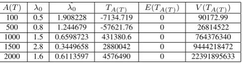
For both A(T)andD(T)takes value 100,500,1000,1500,2000with different values of λ0 = 0.5,0.8,1.5,2.8,1.6 and

µ0= 0.6,0.9,2.5,1.7,2.1respectively. The estimated value ofλ0andµ0was computed using maximum likelihood

[image:7.595.192.418.87.233.2]

estima-tion method. When there is a change occurs in parameterλandµat some pointl, the test statistic and it’s mean and variance value are derived. The simulation results are given in the Table-1 and Table-2 respectively.

Table 1.When change in parameterλ

A(T) λ0 λ0ˆ TA(T) E(TA(T)) V(TA(T)) 100 0.5 1.908228 -7134.719 0 90172.99 500 0.8 1.244679 -57621.76 0 26814522 1000 1.5 0.6598723 431380.6 0 764376340 1500 2.8 0.3449658 2880042 0 9444218472 2000 1.6 0.6113597 4576490 0 22391895633

Table 2.When change in parameterµ

D(T) µ0 µ0ˆ TD(T) E(TD(T)) V(TD(T)) 100 0.6 1.581461 -3914.184 0 131286.5 500 0.9 1.093193 -14916.91 0 34760907 1000 2.5 0.3866171 1094239 0 2226716433 1500 1.7 0.598574 1212004 0 3136768081 2000 2.1 0.4790627 2400702 0 7437162079

Acknowledgments

The work is supported by University Grants Commission under the head′′M ajorResearchP roject′′.

REFERENCES

[1] Acharya, S.K(1999).On normal approximation for maximum likelihood estimation from single server queues, Queue-ing System.31,207−216.

[image:7.595.185.429.469.533.2]

[3] Basawa, I.V. Bhat, U.N and Robert Lund (1996).Maximum likelihood estimation for single server queues from waiting time data,Queueing Systems.24,155−167

[4] Basawa, I.V. and Prabhu, N.U.(1981).Estimation in single server queues,Naval Res. Logist.28,475−487. [5] Basawa, I.V. and Prabhu, N.U. (1988).Large sample inference from single server queues, Queueing Systems. 3,

288−304

[6] Bhat,U.N. and Rao, S.S.(1987).Statistical Analysis of Queueing Systems,Queueing Systems.1,217−247

[7] Brown, R.L., Durbin, J., and evans, J. M.(1975).Tcheniques for testing the constancy of regression relationships over time with disscussion,Journal of the Royal Statistical Society B.37,149−192.

[8] Chernoff, H. and Zacks, S.(1964).Estimating the current mean of a normal distribution which is subject to changes in time, Annals of Mathematical Statistics.35,999−1018.

[9] Chen, J and Gupta, A.K.(2000).Parametric statistical change point analysis,Birkh¨auser, Boston.

[10] Clerke, A. B.(1957).Maximum Likelihood Estimates in a simple queue,Annal. Math. Stat.28,1036−1040.

[11] Kander, Z. and Zacks, S.(1966).Test Procedures for possible changes in parameters of Statistical distributions oc-curing at unknown time pointsAnnals of Mathematical Statistics,37,1196−1210.

[12] Kelly,F.P(1979).Reversibility and Stochastic Networks,Wiley, New York

[13] Krishnaiah, P. R. and Miao,B.Q(1988).Review about estimation of change points (P.R. krishnaiah and C.R.Rao, Eds.) handbook of statistics.7,Elsevier,Amsterdam375−402

[14] Lemoine, A. J.(1977)Networks of Queue- A Survey of Equilibrium Analysis,Manage. Sci.24,464−481

[15] Thiruvaiyaru, D and Basawa, I.V.(1991)Estimation For a Class of Simple Queueing Networks,Queueing Systems9

,301−312

[16] Thiruvaiyaru, D and Basawa, I.V.(1992)Emperical bayes estimation for queueing systems and networks,Queueing Systems11,179−202

[17] Wichern, D.W., Miller, R.B., and Hsu, D.A (1976)changes of varience in first order autoregressive time series models with an applications,Applied Statistics.25,248−356