BDF-
α
: A Multistep Method with Numerical
Damping Control
Elisabete Alberdi Celaya
1,∗,
Juan Jos´
e Anza
21Department of Applied Mathematics, EUIT de Minas y Obras P´ublicas, Universidad del Pa´ıs Vasco UPV/EHU, Bilbao, 48013, Spain
2Department of Applied Mathematics, ETS de Ingenier´ıa de Bilbao, Universidad del Pa´ıs Vasco UPV/EHU, Bilbao, 48013, Spain
∗Corresponding Author: [email protected]
Copyright c⃝2013 Horizon Research Publishing All rights reserved.
Abstract
When solving numerically the stiff second order ODE system obtained after semidiscretizing the wave-type partial differential equation (PDE) with the finite element method (FEM), and similarly to theHHT-α method, which allows the numerical damping of the undesirable high frequency modes associated to FEM semidiscretization, we have constructed a modification of the 2-order BDF method (the BDF2 method), which we have called BDF-α. This new method is second-order accurate and with a smaller local truncation error than the BDF2, it is unconditionally stable for some values ofαand it permits a parametric control of numerical dissipation.
Keywords
BDF, numerical dissipation, amplification matrix, stability1
Introduction
The second order Ordinary Differential Equation (ODE) system obtained after semidiscretizing the wave-type partial differential equation (PDE) with the finite element method (FEM) shows strong numerical stiffness. Its resolution requires the use of numerical methods with good stability properties and controlled numerical dissipation in the high-frequency range.
Some of the methods developed in the linear range are shown in [1]. Time-stepping algorithms such as the Collocation method [2], the Wilson method [3], the HHT-α method [4], the Houbolt method [5], or more recent works as the generalized-alfa method [6] are some of the methods commonly used.
The development of similar methods for nonlinear problems is more recent and it has been originated by the presence of numerical instabilities when solving nonlinear problems by methods which are unconditionally stable in the linear range. Generally, this instablities are due to the increase of energy of the discrete system and this is the reason why the formulation of energy-momentum conserving schemes, [7] and [8], and Energy Dissipative, Momentum Conserving schemes, EDMC [9, 10], have been created.
In this paper, we work in the linear range and we formulate a new method called BDF-α, which is second-order accurate, unconditionally stable for some values of the parameterαand permits a parametric control of numerical dissipation.
2
BDF methods
We will consider the next initial value problem (IVP):
y′(t) =f(t, y(t)), y(t0) =y0 (1)
whereT = [t0, tn] is a finite interval and y:[t0, tn]→Rmand f:[t0, tn]xRm→Rmare continuous functions. The Backward Differentiation Formulae (BDF) were proposed by Gear[11]. They are linear multistep methods useful to solve ODEs of order 1, such as (1). Since they were introduced, the Backward Differentiation Formulae have been widely used due to their good stability properties for solving stiff problems. The BDF of orderkcan be expressed as follows in terms of backward differences:
k
∑
j=1
1
j∇ jy
where: ∇yn+k =yn+k−yn+k−1 and∇jyn+k =∇
( ∇j−1y
n+k
)
. Backward differences verify the next expression:
∇j+1y
n+k=∇jyn+k− ∇jyn+k−1 (3)
Developing the backward differences of expression (2) we get this equivalent expression for the BDFs: k
∑
j=0
αjyn+j=hfn+k (4)
From (4), it is easily deduced that BDFs are linear multistep methods which respond to the general form: k
∑
j=0
αjyn+j=h k
∑
j=0
βjfn+j (5)
Where the constantsαj are chosen in order to verify the order condition, that says that the multistep method will be of orderpif the next condition is satisfied [12, 13]:
Ci= 0, for 1≤q≤p and Cp+1̸= 0
C0=
∑k i=0αi C1=
∑k
i=0iαi−
∑k i=0βi Cq =q1!
(∑k i=0i
qα i
)
− 1
(q−1)!
(∑k i=0i
q−1β
i
) q≥2
(6)
The BDFs are unconditionally stable for orders 1 and 2. The stability properties of the BDFs and their error constants can be calculated following the formulae given in [11, 12, 14]. The A(α)-stability of the BDFs [15, 16] and their error constants can be seen in Table 1.
Table 1. A(α)-stability and error constants of the BDFs.
order 1 2 3 4 5 6
α 90 90 86.03 73.35 51.84 17.84 C -1/2 -1/3 -1/4 -1/5 -1/6 -1/7
If we are interested in studying the amplification factor of the BDFs, the method has to be applied to the test equationy′=λy and we have to rewrite the result using the form:
Xn+k=AXn+k−1 (7)
whereXn+k = (yn+1, yn+2, ..., yn+k)t,Xn+k−1= (yn, yn+1, ..., yn+k−1)tandAis a square matrix of dimensionkxk.
Eigenvalues of matrixAare calculated and the largest one in module is the one we are interested in, which is the spectral radius:
ρ(A) =max{|λi|:λi eigenvalue of A} (8)
The spectral radius is closely connected to the stability of the method and ρ(A) ≤ 1 is required to prevent amplification ofAn asnbecomes large.
When working with second order ODEs, we have to consider their test equationd′′+ω2d= 0, which represents
an undamped vibrating physical system with natural frequency f = ω/(2π). Transforming this equation in its equivalent system of two first order ODEs we get:
( d d′
)′
=
(
0 1
−ω2 0
) ( d d′
)
(9)
System (9) can be uncoupled in two independent equations of the form:
y′=±iωy (10)
and the application of the general theory, (7) and (8), to the second order problemd′′+ω2d= 0 is equivalent to apply this theory to the first order test equationy′ =λy, but now taking into account thatλ takes the specific valueλ=iω.
1 2 3 4 5 6
BDF1 BDF2
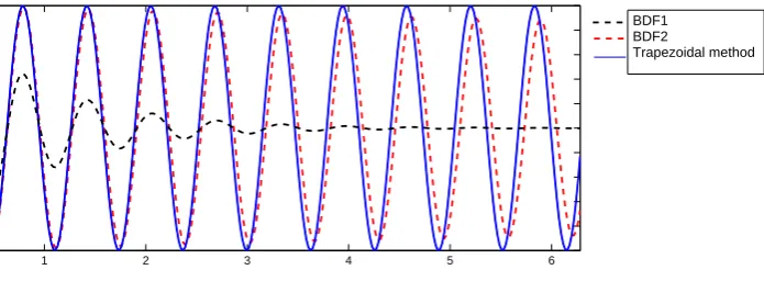
[image:3.595.150.498.61.189.2]Trapezoidal method
Figure 1. Numerical damping of some methods applied toy′′=−102y, (y(0), y′(0)) = (0,1), (300 steps).
Example for calculating the amplification matrix of BDFs
As an example, we have applied this procedure to the BDF4, which expression is given by:
yn+4−
48 25yn+3+
36 25yn+2−
16 25yn+1+
3 25yn =h
12
25fn+4 (11)
We will apply the method given by (11) to the test equationy′=λy, reaching the following expression:
yn+4−
48 25yn+3+
36 25yn+2−
16 25yn+1+
3 25yn = ˆh
12
25yn+4 (12)
where: ˆh=λh. Expression (12) can be written in matrix form as:
A1·Xn+1=A2·Xn⇒Xn+1=A−11A2Xn (13)
where:
A1=
1 0 0 0
0 1 0 0
0 0 1 0
0 0 0 1−1225ˆh
, A2=
0 1 0 0
0 0 1 0
0 0 0 1
−3 25
16 25 −
36 25
48 25
Xn = (yn, yn+1, yn+2, yn+3)
t
, Xn+1= (yn+1, yn+2, yn+3, yn+4)
t ,
(14)
And matrix A=A−11A2 is the amplification matrix of the method (11).
The stability regionS of a numerical method is the set of values ˆh∈Cfor which the spectral radius is less than or equal to one: S =
{
ˆ
h∈C:ρ(A(ˆh))≤1
}
. Applying this condition to the amplification matrix A of the BDF methods, their stability regions are obtained as it is shown in Figure 2.
−10 −5 0 5 10 15 20 −15i
−10i −5i 0 5i 10i 15i
BDF2 BDF3
BDF4 BDF5
[image:3.595.197.384.560.748.2]BDF1
Figure 2. Stability regions of the BDFs (exterior to the curves).
10−2 10−1 100 101 102 103 104 0
0.2 0.4 0.6 0.8 1 1.2 1.4
h/T
ρ
α (α=−0.05) Newmark(β=0.3025,γ=0.6)
α (α=−0.3)
Collocation
(γ=0.5,β=0.16,θ=1.514951)
BDF3
BDF5 BDF2
BDF1
Houbolt
BDF4
HHT−
[image:4.595.160.446.66.301.2]HHT−
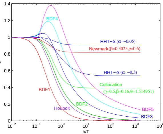
Figure 3. Spectral radii of the BDFs and other methods.
caseλ=iω. Following this condition, the dependence of the spectral radius on ωh/(2π) = h/T can be obtained for BDF methods and others as it is shown in Figure 3.
It can be seen that the spectral radii of the BDFs tend to zero whenh/T →+∞. It can also be observed that in the case of BDFs of orders 3, 4 and 5, there is a zone in which the spectral radius becomes greater than one. This is because these methods are not stable in a certain zone near to and in the imaginary axis.
When solving a second order ODE, measures of accuracy such as the algorithmic damping ratio ¯ξ and the relative period error ( ¯T−T)/T are relevant, see Figure 1. The first one ¯ξ, says how much decays the amplitude and the second measures how much periods are elongated or shortened. It is difficult to obtain analytical expressions for ¯ξand ( ¯T−T)/T but they can be calculated by computer evaluation.
When solving second order ODEs that come from the FEM semidiscretization of the wave-type PDE, the higher modes of these equations are artifacts of the discretization process and they are not representative of the behaviour of the governing PDE. So it is convenient to introduce algorithmic damping to remove the participation of high-frecuency modal components. Even though the minimum value that BDFs show forρ∞ = limh/T→∞ρ(A) is the most effective in removing the participation of high-frecuency modal components, it is more convenient to have an algorithm which permits a parametric control of numerical dissipation, allowing the participation of the medium frequencies. Figure 3 shows how the parametric control α=−0.3 of the HHT-αmethod decreases the medium range frequency numerical damping with respect to the stable BDFs, while maintaining a low spectral radius in the high range, which is enough to dissipate quickly this frequency components.
We are interested in creating a method with the same properties as the HHT-αbut taking as basis the BDFs. Next we will review direct methods for second order ODEs and in particular the Newmark parametric family in which HHT-αis based.
3
Linear multistep methods for second order ODEs
Consider the second order initial value problem:
y′′=f(t, y, y′), y(t0) =η, y′(t0) = ˆη (15)
whereT = [t0, tn] is a finite interval and y:[t0, tn]→Rmand f:[t0, tn]xRm→Rm are continuous functions. Writing equation (15) as a first order system and applying a linear ˜k-step method (5):
{∑˜k
j=0αjyn+j =h
∑k˜
j=0βjyn′+j
∑˜k
j=0αjy′n+j =h
∑k˜
j=0βjf(tn+j, yn+j, y′n+j)
(16)
An elimination of
{
yn′+j:j= 0,1, ...,˜k }
in (16) results [14]: k
∑
j=0
ˆ
αjyn+j=h2 k
∑
j=0
ˆ
wherek= 2˜k.
Expression (17) corresponds to a linear multistep method for second order differential equations, which is similar to first order equations but with different coefficients and appearing the factor h2 instead of the factor hof the
first order ODEs.
HHT-αmethod can be reduced to (17) form, and general properties of second order ODEs multistep methods can be used to study its properties. HHT-αmethod is an extension of the Newmark family which in turn can be introduced based on the trapezoidal method.
In computational mechanics, the second order linear ODE takes the form:
ma+cv+kd=f(t) (18)
which corresponds to a mass-spring-damper system, where m is the mass, k the spring constant, c the damping coefficient,v=d′ the velocity anda=d′′ the acceleration.
Converting the second order equation (18) into a first order system:
( d v
)′
=
( v a )
(19) whereaverifies (18), and applying the trapezoidal method to it, we get:
dn+1=dn+
vn+vn+1
2 h
vn+1=vn+
an+an+1
2 h
(20)
It can be observed that in relations (20), the displacement and the velocity are updated using the average velocity and acceleration of the instants tn andtn+1, respectively. By substituting the second formula of (20) in
the first one, the exact formula of the uniformly accelerated motion is obtained:
dn+1=dn+vnh+
(an
2 +
an+1
2
)h2
2 (21)
If instead of the average acceleration, two weighted means are considered, taking in one of them the parameter 2β and in the other one the parameterγ, we obtain the biparametric family of the Newmark method [17]:
dn+1=dn+ ∆tvn+∆t 2
2 [(1−2β)an+ 2βan+1]
vn+1=vn+ ∆t[(1−γ)an+γan+1]
man+1+cvn+1+kdn+1=fn+1
(22)
where β andγ are free parameters which govern the accuracy, stability and numerical dissipation of Newmark’s algorithm.
With the purpose of studying the stability and the numerical damping of the method, we apply the method to the test equation d′′+ω2d= 0, where w =√k/m. In this case, (22) can be succinctly written in this recursive way:
Xn+1=AXn (23)
where: Xn+i=
(
dn+i, hvn+i, h2an+i
)T
fori= 0,1,h= ∆t andAis given by: A=A1−1·A2, and:
A1=
10 0h1 −−h1βγ
ω2 0 1
h2
, A2=
1 1
1 2 −β
0 h1 1h(1−γ)
0 0 0
The system (23) can be reduced to a difference equation in the displacementes, which takes the form of a linear multistep method for second order differential equations (17):
2
∑
i=0
αidn+i=h2
2
∑
i=0
βid′′n+i (24)
where the coefficientsαj,βj are given by:
α0= 1, β0=−γ+β+12
α1=−2, β1=−2β+γ+12
α2= 1, β2=β
(25)
The order of the method can be calculated by applying the order conditions for linear multistep methods of the type (24) [18]. The method results second-order accurate whenγ= 1/2, [1, 17]. The method is unstable when
γ < 1
2 and it is unconditionally stable when 1
2 ≤γ≤2β. High frequency dissipation is achieved when:
β=
( γ+1
2
)2
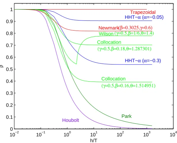
In the second-order accurate Newmark method (γ= 1/2),β ≥1/4 retains unconditional stability. If in addition, high frequency dissipation is requiered,β = 1/4 has to be verified. In this case, Newmark’s method becomes the trapezoidal method, and although it verifies the high frequency dissipation condition (26), high modes are not damped asρ∞= 1, see Figure 4. So, second-order accurate condition does not allow numerical dissipation.
The HHT-α method is a modification made to the Newmark method, with the aim of obtaining numerical dissipation in the high frequencies while retaining the order and stability conditions. This method was proposed by Hilber-Hughes-Taylor[4] and it is also known as HHT or theα-method. The method consists of maintaining the two first expressions of the Newmark method (22) and varying the third expression. That is to say, modifying the expression of the time-discrete equation of motion with a new parameterαas follows:
man+1+cvn+1+α+kdn+1+α=f(tn+1+α) (27)
where:
dn+1+α= (1 +α)dn+1−αdn vn+1+α= (1 +α)vn+1−αvn tn+1+α= (1 +α)tn+1−αtn
(28)
In the case that α= 0, the HHT-αmethod is reduced to Newmark’s method.
When applied tod′′+ω2d= 0, the method takes the recursive form (23), whereA=A1−1·A2is the amplification
matrix and:
A1=
10 01h −−1hβγ ω2(1 +α) 0 1
h2
, A2=
1 1
1 2−β
0 1
h
1
h(1−γ)
ω2α 0 0
Similarly to Newmark, HHT-αmethod can also be reduced to a three-step linear multistep method for second order differential equations (17):
3
∑
i=0
αidn+i=h2
3
∑
i=0
βid′′n+i (29)
where the coefficientsαj, βj are given by:
α0= 0, β0=γα−12α−βα
α1= 1, β1=−2γα+ 3βα−γ+β+12
α2=−2, β2=β(−3α−2) +
( γ+1
2
)
(1 +α)
α3= 1, β3=β+βα
(30)
The method is second-order accurate when γ = 1−22α and if α∈[−13,0],β = (1−4α)2 the HHT-αmethod is a two-order method, unconditionally stable and high frecuency dissipation can be obtained.
In Figure 4 we can see the spectral radii of Newmark and HHT-αmethods together with the spectral radii of other typical methods used in computational mechanics, such us, Houbolt’s method, Collocation method (among them the Wilson method which is a concrete case of the Collocation method) and Park’s method [1, 2, 5]. In this figure we can see that the spectral radii of Houbolt’s and Park’s method tend to zero as ∆t/T → ∞ which is typical in backward-differences schemes. It can also be seen, how the A-stable HHT-αmethod whenα∈[−13,0], dampens the high modes more strongly as the value ofαdecreases, but in a much smoother way than the BDFs for the medium range of frequencies (see Figure 3).
4
BDF-
α
We have seen in Figure 3 that the spectral radii of the BDF2 tends to zero when h/T → +∞. This method has strong dissipation of medium and high frequencies and our aim is to construct a parametrized method wich allows numerical damping control, in the same way that the HHT-αdoes. The BDF2 is a two-order and A-stable method given by the next expression:
3
2yn+2−2yn+1+ 1
2yn=hfn+2 (31)
We will make some considerations about the modification that have arisen:
10−2 10−1 100 101 102 103 104 0
0.1 0.2 0.3 0.4 0.5 0.6 0.7 0.8 0.9 1
h/T
ρ
Collocation
(γ=0.5,β=0.16,θ=1.514951)
Houbolt
(γ=0.5,β=0.18,θ=1.287301) (γ=0.5,β=1/6,θ=1.4) Wilson
Collocation
HHT−α (α=−0.05)
HHT−α (α=−0.3) (β=0.3025,γ=0.6)
Newmark
Trapezoidal
[image:7.595.143.433.67.301.2]Park
Figure 4. Spectral radii of some methods.
2. The first modification which we have been considering consisted of adjusting each addend of BDF2. In this way a general expression in which y, y′ evaluated in tn, tn+1, tn+2 is reached. That is to say, we have been
trying with an expression like:
α1yn+2+α2yn+1+α3yn=β1fn+2+β2fn+1+β3fn (32) We have dismissed this possibility (32), mainly for two reasons. The first one is that this expression’s origin is not equivalent to the couple Newmark&HHT-α. And the second one is that even though it is possible to achieve order 2 using (32), expression (32) has all the addends that appear in methods such as Adams Moulton and BDF2, so we would be creating a linear combination that we are not interested in.
{
Adams Moulton (k= 2):yn+2=yn+1+h
(5
12fn+2+ 2 3fn+1−
1 12fn
)
BDF (k= 2): 32yn+2−2yn+1+12yn=hfn+2
(33)
3. The HHT-αmethod, which was constructed taking the Newmark method as its basis, verifies all the charac-teristics that we want for our method, and the form in which it was constructed may help us in our way of thinking about the most convenient form that the new method should have. Newmark’s method is given by the expressions (22). In the method HHT-α, the first two expressions of (22) are maintained and the third one is adjusted:
Newmark’s form: man+1+cvn+1+kdn+1=fn+1 (34)
HHT-α’s form: man+1+ (1 +α)cvn+1−αcvn+ (1 +α)kdn+1−αkdn=f(tn+1+α) (35) 4. A possible formula which we have tried consisted of adjusting uniquely the right-hand side of expression (31):
3
2yn+2−2yn+1+ 1
2yn=h[(1 +α)fn+2−αfn+1] (36) The problem that we have found is that the numerical method given by the expression (36) has only order 1 whenα̸= 0 and whenα= 0, expression (36) is reduced to the BDF2.
5. Finally, we have considered a modification with three free parametersα,β andγ which can be expressed as follows, in order to clearly see the calculations required:
3
2((1 +β)yn+2−βyn+1)−2 ((1 +γ)yn+1−γyn) + 1
2yn=h((1 +α)fn+2−αfn+1) (37) Reordering terms in (37) we obtain the next expression for the modification of the BDF2 that we require:
yn+2
3
2(1 +β) +yn+1
( −3
2β−2(1 +γ)
)
+yn
(
2γ+1 2
)
This expression can be written in the following abreviate way, which corresponds with the standard form of a linear multistep method or linear k-step method (5):
2
∑
j=0
αjyn+j=h
2
∑
j=0
βjfn+j
where: {
α2= 32(1 +β), α1=−23β−2(1 +γ), α0= 2γ+12
β2= 1 +α, β1=−α, β0= 0
(39)
4.1
Order and error constant
Theorem. The method given by the expression (38) will be of order 2 if the constants α, β, γ verify the following conditions: α= 32β= 2γ.
Proof.
We have already said that BDF-α’s expression (38) can be written as a multistep method (5) where the values of the constants are given by (39). So the BDF-αmethod is a linear multistep method, specifically a 2-step method. This method will be of order 2 ifC0=C1=C2= 0 and C3̸= 0 [12, 13], where theCi constants are given by (6). We substitute the values of (39) in the expressions of (6) and we get:
C0=
∑2
i=0αi= 0
C1=
∑2
i=0iαi−
∑2
i=0βi=−2γ+32β C2= 2!1
(∑2
i=0i 2α
i
) −(∑2
i=0iβi
)
=−γ+94β−α C3= 3!1
(∑2
i=0i 3α
i
) − 1
2!
(∑2
i=0i 2β
i
)
= 74β−13−γ3 −32α
(40)
We already have C0 = 0. The method will be of order 2 if C1 =C2 = 0 and this happens when α, β, γ are
chosen in this way: α= 32β= 2γ.
We can conclude by saying that the expression of the 2-order BDF-αis written as follows:
(
3 2 +α
)
yn+2+ (−2−2α)yn+1+
(
1 2+α
)
yn=h(1 +α)fn+2−hαfn+1 (41)
Observe that when α= 0 we have the BDF2 method and for α =−0.5 the trapezoidal method is obtained. Whenα= 1−aa wherea∈Rthe method (41) is the same as the A-BDF method [19] fork= 2.
The local truncation error of the method BDF-αis given by the next expression:
LT E=Ch3y′′′(tn) +O(h4) (42)
And the error constant C of the method is given by:
C= C3
σ(1) (43)
where, after substituting the second order conditionα= 32β= 2γ inC3, we get:
C3=
7 4β−
1 3−
γ
3 − 3 2α=
−2−3α
6 (44)
andσ(r) is one of the two characteristic polynomials of the method [11, 12, 14] given by:
σ(r) =
2
∑
j=0
βjrj =−αr+ (1 +α)r2⇒σ(1) =−α+ 1 +α= 1 (45)
By substituting (44) and (45) in (43), the error constant of the BDF-αmethod is obtained:
C= −2−3α
6 (46)
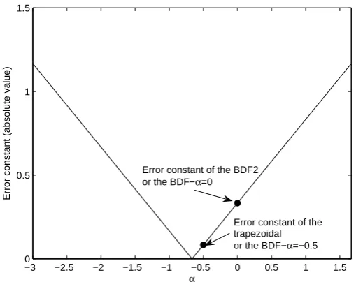
Whenα= 0 the value of the error constant isC=−13 which, as expected, is the error constant of the BDF2 method. In the caseα=−0.5, we have the trapezoidal method and we get the well-known error constant:C=−121. The value of the error constant in relation to the value ofαis shown in Figure 5. In Section 4.2 we will see that the BDF-αmethod is A-stable forα≥ −0.5, so, the BDF-αthat corresponds toα=−0.5 is the one that has the smallest error constant, which corresponds to the trapezoidal rule. So, the theorem of Dhalquist (1963) is verified; which says that a multistep A-stable method is of orderp≤2, being the trapezoidal rule the second order A-stable method with smallest error constant [15, 20].
So, we have that the BDF-αis second-order accurate and it has a smaller error constant than the BDF2 for
−3 −2.5 −2 −1.5 −1 −0.5 0 0.5 1 1.5 0
0.5 1 1.5
α
Error constant (absolute value)
Error constant of the trapezoidal or the BDF−α=−0.5 Error constant of the BDF2
[image:9.595.152.407.54.256.2]or the BDF−α=0
Figure 5. Absolute value of the error constant of the method BDF-α.
4.2
Stability regions
The region of absolute stability of the overall method BDF-αis found using Schur’s theorem [18]. To do this, we will apply the method BDF-αto the test equationy′ =λy. That is to say,hfj =hλyj is introduced in expression
(41). (
3 2+α
)
yn+2+ (−2−2α)yn+1+
(
1 2 +α
)
yn = ˆh(1 +α)yn+2−ˆhαyn+1 (47)
where ˆh=λh.
We will setyp=rp to obtain the characteristic polynomial and after taking out ˆh, we get: ˆ
h=
(3
2+α
)
r2+ (−2−2α)r+(12+α)
(1 +α)r2−αr (48)
By substitutingr=eiθ in (48) we get the expression of the boundary of the stability regions:
ˆ
h(θ) =
(1 + 2α)(cosθ−1)2+isinθ[(1 + 2α)(1−cosθ) + 1 1+α
]
(1 +α)
[(
cosθ−1+αα )2
+sin2θ
] (49)
Forα≥ −0.5 the denominator of ˆh(θ) is bounded from below by a positive constant. So, having fixedα≥ −0.5, for a sufficiently large real number which depends onαand independent ofθ,R(α)∈R, next expression is verified:
0≤Re(ˆh(θ))≤R(α) (50)
The boundary of the stability region ˆh(θ) lies in a compact subset of the right half-planeC+. For any ˆh∈C−,
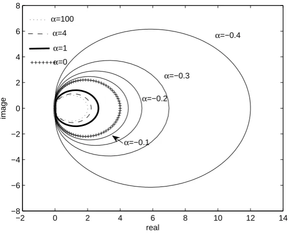
absolute stability is achieved and for continuity reasons this implies thatC−belongs to the stability region, which means that the method is A-stable whenα∈[−0.5,+∞). Figure 6 shows some stability regions of the BDF-αfor some values ofα.
4.3
Amplification matrix
After applying the BDF-αmethod to the test equation, the following expression is obtained:
Xn+1=AXn (51)
where:
Xn+1=
( yn+1
yn+2
) , Xn =
( yn
yn+1
)
, A=A−11A2
A1=
(
1 0
0 32+α−ˆh(1 +α)
) , A2=
(
0 1
−1
2 −α 2 + 2α−ˆhα
)
, ˆh=λh
(52)
Matrix A is the amplification matrix whose eigenvalues are given by:
λ1,2=
−2−2α+ ˆhα± √
ˆ
h2α2+ 2ˆh(α+ 1) + 1
−2 0 2 4 6 8 10 12 14 −8
−6 −4 −2 0 2 4 6 8
real
image
α=−0.4
α=−0.3
α=−0.2
α=−0.1 α=0
α=1 α=4 α=100
[image:10.595.158.447.67.300.2]+++++++
Figure 6. Stability regions of the BDF-α(exterior to the curves).
The characterization of the numerical dissipation of the method in function of the parameter α requires the study of the limit of the spectral radius when ˆh→ ∞:
ρ∞= lim
ˆ
h→∞
max{|λ1, λ2|}= max
{ α2 + 2± |αα|
}=
−2α
−2−2α >1, α∈(−∞,−1) −2α
2+2α, α∈(−1,0]
2α
2+2α <1, α∈[0,+∞)
(54)
Whenα∈(−∞,−1),ρ∞ is greater than 1; we have already seen that in this case the method is not A-stable. In the intervalα∈(−1,0] expression (54) takes these values:
ρ∞= −2α 2 + 2α =
−2α
2+2α>1, α∈(−1,−0.5) 1, α=−0.5
−2α
2+2α<1, α∈[−0.5,0)
(55)
Again, we see that ρ∞>1 when α∈(−1,−0.5).
For the A-stable BDF-αmethod, and this happens whenα≥ −0.5 as has been proved in Section 4.2, the value ofρ∞is given by:
ρ∞=
1, α=−0.5
−2α
2+2α <1, α∈[−0.5,0)
2α
2+2α <1, α∈[0,+∞)
(56)
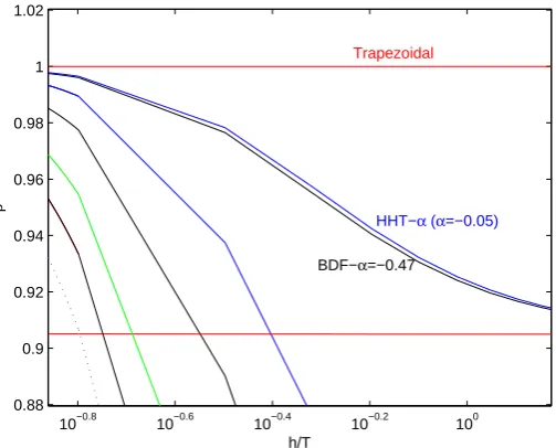
and from this last expression it is easy to conclude that in the A-stable BDF-α method,ρ∞ takes all the values of the interval (0,1]. This means that having fixed a value for ρ∞ ∈ (0,1], it is possible to obtain a second-order accurate and A-stable BDF-αmethod with that spectral radius in ˆh→ ∞. So, our new method permits a parametric control of numerical dissipation. In Figure 7 some spectral radii of BDF-αare shown.
We have also calculated the value of the parameterαof the method BDF-α, which has the same spectral radius as the method HHT-α when h/T → +∞ for HHT-α = −0.05 and HHT-α = −0.3. For HHT-α = −0.05 the spectral radius whenh/T →+∞is ρ= 0.90476. The same value is obtained inh/T →+∞for α1 =−0.475065
and α2 = 9.50 of the method BDF-α. The Figures of the spectral radii are similar in these cases although it
can be seen in Figure 8 that they are not exactly the same. In the same way, the value of the spectral radius in HHT-α = −0.3 is ρ = 0.53846. The method BDF-α for α1 = −0.35 and α2 = 1.17 has the same spectral
radius in h/T → +∞ as the HHT-α = −0.3. In both cases, HHT-α= −0.05 and HHT-α= −0.3, the BDF-α
couples obtained are second-order accurate and unconditionally stable, but the methods BDF-α2= 9.50 and
BDF-α2= 1.17 have a lower spectral radius in the medium range frequency with respect to the HHT-α. So, the methods
BDF-α1=−0.475065 and BDF-α1=−0.35 are more similar to their respective HHT-αmethods.
4.4
Relative period error and algorithmic damping
10−2 10−1 100 101 102 103 104 0
0.2 0.4 0.6 0.8 1
h/T
ρ
Trapezoidal
HHT−α (α=−0.05) BDF−α=9.50 BDF−α=−0.47
HHT−α (α=−0.3)
BDF−α=−0.35
Collocation (γ=0.5,β=0.16,θ=1.514951)
BDF−α=0 Houbolt
[image:11.595.162.415.66.270.2]BDF−α=1.17
Figure 7. Some spectral radii of the method BDF-αand others.
10−0.8 10−0.6 10−0.4 10−0.2 100
0.88 0.9 0.92 0.94 0.96 0.98 1 1.02
h/T
ρ
HHT−α (α=−0.05) Trapezoidal
[image:11.595.160.412.321.524.2]BDF−α=−0.47
Figure 8. Some spectral radii of the method BDF-αand others (closer image).
0 0.05 0.1 0.15 0.2 0.25 0.3 0.35 0.4
0 0.1 0.2 0.3 0.4 0.5 0.6 0.7 0.8 0.9
h/T
ξ
BDF−α=1.17
BDF−α=0
BDF−α=−0.35 l
BDF−α=9.50
TrapezoidalBDF−α=−0.475065
0 0.05 0.1 0.15 0.2 0.25 0.3 0.35 0.4
0 0.01 0.02 0.03 0.04 0.05 0.06 0.07 0.08 0.09 0.1
h/T
ξ
BDF−α=0
BDF−α=−0.35
l
Houbolt
HHT−α (α=−0.3) Collocation
(γ=0.5,β=0.16, θ=1.514951)
BDF−α=−0.475065
HHT−α (α=−0.05) Trapezoidal
Figure 9. Algorithmic damping of BDF-αmethod and others.
[image:11.595.80.489.576.747.2]0 0.05 0.1 0.15 0.2 0.25 0.3 0.35 0.4 0
0.2 0.4 0.6 0.8 1 1.2
h/T
(T−T)/T
I
Trapezoidal
BDF−α=0
BDF−α=−0.35
BDF−α=−0.47
BDF−α=1.17
BDF−α=9.50
0 0.05 0.1 0.15 0.2 0.25 0.3 0.35 0.4
0 0.05 0.1 0.15 0.2 0.25 0.3 0.35 0.4 0.45 0.5
h/T
(T−T)/T
I
Trapezoidal
BDF−α=0
BDF−α=−0.35
BDF−α=−0.47 Houbolt
HHT−α (α=−0.3)
[image:12.595.92.510.64.224.2]HHT−α (α=−0.05)
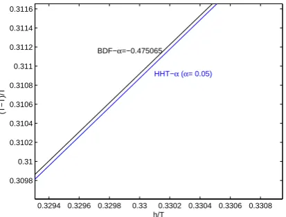
Figure 10. Relative period errors of the BDF-αmethod.
0.3294 0.3296 0.3298 0.33 0.3302 0.3304 0.3306 0.3308 0.3098
0.31 0.3102 0.3104 0.3106 0.3108 0.311 0.3112 0.3114 0.3116
h/T
(T−T)/T
HHT−α (α= 0.05) BDF−α=−0.475065
I
Figure 11. Relative period errors of the BDF-αmethod (closer image).
The trapezoidal rule is again, the one with the smallest relative period error. It can also be seen that figures of the algorithmic damping of the method HHT forα=−0.05 andα=−0.3 are smaller than the ones corresponding to BDF-αwith α=−0.475065 andα=−0.35, which were the couple of methods that in h/T →+∞have the same spectral radius. The same occurs with the relative errors in period as can be seen in Figures 10 and 11: the ones corresponding to the HHT-αmethods are smaller than the ones of the BDF-αin the same couples.
5
Concluding remarks
The BDF-αmethod is a parametrized second-order accurate multistep method, A-stable whenα∈[−0.5,+∞) and which allows controlled numerical dissipation in the medium and high-frequency range when applied to second order ODEs modelling vibratory systems. This is a desirable property when dealing with second order ODE systems associated to the FEM semidiscretization of the wave-type PDEs.
In addition, the BDF-αmethod improves the constant error of the BDF2 and its spectral radiiρ∞ sweeps the whole interval [0,1] improving the numerical damping control offered by the HHT-αmethod.
REFERENCES
[1] Thomas J. R. Hughes, The finite element method. Linear Static and dynamic finite element analysis, Prentice-Hall International Editions, New Jersey, 1987.
[2] Hans M. Hilber, Thomas J.R. Hughes, Collocation, dissipation and overshoot for time integration schemes in structural dynamics,Earthq. Eng. Struct. Dyn., Vol.6, 99-117, 1978.
[3] E.L. Wilson, A computer program for the dynamic stress analysis of underground structures,SEL Report, Vol.68, No.1, 1968.
[image:12.595.194.401.269.426.2][5] Ian Gladwell, Ruth Thomas, Stability properties of the Newmark, Houbolt and Wilson θ methods, Int. J. Numer. Anal. Methods Geomech., Vol.4, 143-158, 1980.
[6] J. Chung, G. M. Hulbert,A time integration algorithm for structural dynamics with improved numerical dissipation: the generalized-αmethod,Journal of Applied Mechanics, Vol.60, 371-375, 1993.
[7] J. C. Simo, N. Tarnow, The discrete energy-momentum method. Conserving algorithms for nonlinear elastodynamics,
ZAMP, Vol.43, 757-793, 1992.
[8] O. Gonzalez, Exact energy-momentum conserving algorithms for general models in nonlinear elasticity,Comput. Meth-ods Appl. Mech. Eng., Vol.190, 1763-1783, 2000.
[9] F. Armero, I. Romero, On the formulation of high-frequency dissipative time stepping algorithms for nonlinear dy-namics. Part I: low order methods for two model problems and nonlinear elastodynamics,Comput. Meth. Appl. Mech. Eng., Vol.190, 2603-2649, 2000.
[10] F. Armero, I. Romero, On the formulation of high-frequency dissipative time stepping algorithms for nonlinear dynam-ics. Part II: second order methods,Comput. Meth. Appl. Mech. Eng., Vol.190, 6783-6824, 2001.
[11] C. William Gear, Numerical initial value problems in Ordinary Differential Equations, Prentice Hall, New Jersey, 1971.
[12] J. C. Butcher, Numerical methods for ordinary differential equations in the 20th century, J. Comput. Appl. Math., Vol.125, 1-29, 2000.
[13] J. D. Lambert, Numerical methods for ordinary differential systems: the initial value problem, John Wiley & Sons, Chichester, 1991.
[14] E. Hairer, S. P. Nørsett, G. Wanner, Solving ordinary differential equations, I, Nonstiff problems, Springer, Berlin, 1993.
[15] E. Hairer, G. Wanner, Solving ordinary differential equations, II, Stiff and Differential Algebraic Problems, Springer, Berlin, 1996.
[16] L.F. Shampine, M.W. Reichelt, The MATLAB ODE suite,SIAM J. Sci. Comput., Vol.18, No.1, 1-22, 1997.
[17] N. M. Newmark, A method of computation for structural dynamics,J. Eng. Mech. Div., ASCE, Vol.85, 67-94, 1959. [18] J. D. Lambert, Computational Methods in Ordinary Differential Equations, Wiley, London, 1973.
[19] Christoph Fredebeul, A-BDF: A generalization of the backward differentiation formulae,SIAM J. Numer. Anal., Vol.35, No.5, 1917-1938, 1998.