Optimization techniques for business process analysis on automotive industry in Malaysia

PROCESS ANALYSIS ON AUTOMOTIVE INDUSTRY IN

MALAYSIA

ABDUL TALIB BON

JEAN MARC OGIER

AHMAD MAHIR RAZALI

PROCEDINGS OF THE 3

rd

INTERNATIONAL BORNEO

BUSINESS PROCESS ANALYSIS ON AUTOMOTIVE

INDUSTRY IN MALAYSIA

O P T I M I Z A T I O N T E C H N I Q U E S F O R BUSINESS P R O C E S S A N A L Y S I S O N

A U T O M O T I V E I N D U S T R Y IN M A L A Y S I A

Abdul Talib Bon, Jean Marc Ogier Department Informatique - Laboratorie L3i

Pole Sciences et Technologie Universite de La Rochelle, F R A N C E [email protected]. [email protected]

Ahmad Mahir Razali

School of Mathematical Sciences Faculty of Science and Technology Universiti Kebangsaan Malaysia, M A L A Y S I A

[email protected]

A B S T R A C T

Optimization is necessary for the control of any business process to achieve better product quality, high productivity with low cost. The beltline moulding process is difficult task due to its low defects, making the material sensitive to reject. The efficient beltline moulding process involves the optimal selection of operating parameters to maximize the number of production while maintaining the required quality limiting beltline surface damage. In this research, objective is to obtain optimum process parameters, which satisfies given limit, minimizes number of defects and maximizes the productivity at the same time. A recently developed optimization algorithm called particle swarm optimization is used to find optimum process parameters. Accordingly, the results indicate that a system where multilayer perceptron is used to model and predict process outputs and particle swarm optimization is used to obtain optimum process parameters can be successfully applied to beltline moulding process through Particle Swarm Optimization (PSO). Results obtained are superior in comparison with Genetic Algorithm (GA) approach.

Keywords: Beltline moulding, Parameters, Particle swarm optimization, Genetic Algorithm, Business Process

1. Introduction

concept of combining Genetic Algorithms (GA) and Particle Swarm Optimization (PSO) simulation is presented in the context of this research. Based on these considerations, conclusions on the current and future role of simulation in business process modelling are presented. Although different authors have formalised different definitions of business processes, an overview of which may be found in (Hlupic and de Vreede 2005), there is a general consensus on some common elements: the process itself, whether it is referred to as a transformation of input, as a work flow, or as a set of activities, its input, and its output, often referred to as value to the customer, or business goal (Hlupic and de Vreede 2005, Hlupic and Robinson 1998).

Particle Swarm Optimization (PSO) is a recently proposed algorithm by R.C Eberhart and James Kennedy in 1995, motivated by social behaviour of organisms such as bird flocking and fish schooling. P S O algorithm is not only a tool for optimization, but also a tool for representing socio cognition of human and artificial agents, based on principles of social psychology. P S O as an optimization tool provides a population-based search procedure in which individuals called particles change their position or state with time. In a P S O system, particles fly around in a multidimensional search space. During flight, each particle adjusts its position according to its own experience, and according to the experience of a neighbouring particle, making use of the best position encountered by itself and its neighbour. Thus, as in modern Gas and memetic algorithms, a P S O system combines local search methods with global search methods, attempting to balance exploration and exploitation.

The P S O Algorithm shares similar characteristics to Genetic Algorithm, however, the manner in which the two algorithms traverse the search space is fundamentally different. Both Genetic Algorithms and Particle Swarm Optimizers share common elements:

1. Both initialize a population in a similar manner.

ii. Both use an evaluation function to determine how fit (good) a potential solution is.

iii. Both are generational, that is both repeat the same set of processes for a predetermined amount of time.

Particle Swarm has two primary operators: Velocity update and Position update. During each generation each particle is accelerated toward the particles previous best position and the global best position. At each iteration a new velocity value for each particle is calculated based on its current velocity, the distance from its previous best position, and the distance f r o m the global best position. The new velocity value is then used to calculate the next position of the particle in the search space. This process is then iterated a set number of times or until a minimum error is achieved.

This study has presented beltline moulding process by using multilayer perceptron modelling and particle swarm optimization. A multilayer perceptron model of beltline moulding was used to determine the optimal number of hidden units to represent the model and particle swarm optimization was used to minimize the Mean square error (MSE) between the actual output and the modelled output. T w o different test cases illustrated that the combined multilayer perceptron and particle swarm optimization system is capable of generating optimal process parameters and can be used successfully in the parameters selection optimization of beltline moulding. Particle swarm optimization is also proved to be an efficient optimization algorithm. For the test cases it yielded optimal parameter around 100 iterations, which take only a little time with today's computers.

2. Literature Review

Each particle keeps track of its coordinates in the problem space which are associated with the best solution (fitness) it has achieved so far. (The fitness value is also stored.) This value is called pbest. Another "best" value that is tracked by the particle swarm optimizer is the best value, obtained so far by any particle in the neighbours of the particle. This location is called Ibest. When a particle takes all the population as its topological neighbours, the best value is a global best and is called gbest.

The particle swarm optimization concept consists of, at each time step, changing the velocity of (accelerating) each particle toward its pbest and Ibest locations (local version of PSO). Acceleration is weighted by a random term, with separate random numbers being generated for acceleration toward pbest and Ibest locations. In past several years, P S O has been successfully applied in many research and application areas. It is demonstrated that P S O gets better results in a faster, cheaper way compared with other methods. Another reason that P S O is attractive is that there are few parameters to adjust. One version, with slight variations, works well in a wide variety of applications. Particle swarm optimization has been used for approaches that can be used across a wide range of applications, as well as for specific applications focused on a specific requirement.

Multilayer perceptron models which are developed for a better understanding of the effects of beltline moulding process and the resultant quality of beltline can be combined with optimization methods in order to determine optimum control parameters for different objectives such as minimizing manufacturing cost or maximizing productivity. Evolutionary computation algorithms such genetic algorithms and particle swarm optimization are usually utilized for optimization of multilayer perceptron based models. Tandon et al (2002) optimized machining parameters in end milling to minimize machining time by combining a feed forward neural network force model with particle swarm optimization.

3. Methodology

Instead of mutation P S O relies on the exchange of information between individuals, called particles, of the population, called swarm. In effect, each particle adjusts its trajectory towards its own previous best position, and towards the best previous position attained by any member of its neighbourhood (Kennedy. J, 1998).

The particles evaluate their positions relative to a goal (fitness) at every iteration, and particles in a local neighbourhood share memories of their "best" positions, then use those memories to adjust their own velocities, and thus subsequent positions. The original formula developed by Kennedy and Eberhart was improved by Shi and Eberhart (1998) with the introduction of an inertia parameter, w, that increases the overall performance of PSO. The best previous position (i.e. the position corresponding to the best function value) of the i-th particle is recorded and represented as Pi = (pa, Pi2 PID), and the position change (velocity) of the i-th particle is Vi = (vn, vi2 viD)- The particles are manipulated according

to the following equations (the superscripts denote the iteration):

where i = 1,2,....,N, and N is the size of the population; % is a constriction factor which is used to control and constrict velocities; co is the inertia weight; c, and c2 are two positive

constants, called the cognitive and social parameter respectively; ril and ri2 are random numbers uniformly distributed within the range [0,1]. Eq. (1) is used to determine the i-th particle's new velocity, at each iteration, while Eq. (2) provides the new position of the i-th particle, adding its new velocity, to its current position. The performance of each particle is measured according to a fitness function, which is problem {dependent. In optimization

xT=x>vT

g a )

problems, the fitness function is usually identical with the objective function under consideration.

The first term on the right hand side of Eq. (1) is the previous velocity of the particle, which enables it to fly in search space. The second and third terms are used to change the velocity of the agent according to pbest and gbest. The iterative approach of P S O can be described as follows:

Step 1: Initial position and velocities of agent are generated. The current position of each particle is set as pbest. The pbest with best value is set as gbest and this value is stored. The next position is evaluated for each particle by using Eq. (1) and (2).

Step 2: The objective function value is calculated for new positions of each particle. If a better position is achieved by an agent, the pbest value is replaced by the current value. As in Step 1, gbest value is selected among p b e s t values. If the new gbest value is better than previous gbest value, the gbest value is replaced by the current gbest value and stored.

Step 3: Steps 1 and 2 are repeated until the iteration number reaches a predetermined iteration number.

Success of P S O depends on the selection of parameters given in Eq (1). Shi and Eberhardt (1998) studied the effects of parameters and concluded that cl and c2 can be taken around the value of 2 independent from problem. Weighting function w is usually utilized according to the following formula,

"Wmax "Wmin „ • , /-,. w = wmax — Hter (3)

1 1 0 / max

where:

wm a x: initial weight

wmm : final weight

itermax : maximum iteration number

iter : current iteration number

Eq. (3) decreases the effect of velocity towards the end of search algorithm, which confines the search in a small area to find optima accurately. The velocity update step in P S O is stochastic due to random numbers generated, which may cause an uncontrolled increase in velocity and therefore instability in search algorithm. In order to prevent this, usually a maximum and a minimum allowable velocity is selected and implemented in the algorithm. In practice, these velocities are taken as [-4.0,+4.0].

The role of the inertia weight, w is considered important for the PSO's convergence behaviour. The inertia weight is employed to control the impact of the previous history of velocities on the current velocity. Thus, the parameter w regulates the trade-off between the global (wide-ranging) and the local (nearby) exploration abilities of the swarm. A large inertia weight facilitates exploration (searching new areas), while a small one tends to facilitate exploitation, i.e. fine tuning the current search area. A proper value for the inertia weight, w provides balance between the global and local exploration ability of the swarm, and, thus results in better solutions.

4. Results and Discussions

4.1 Modelling the data using MLP

For the defects model, the output is the Mean Square Error, M S E of actual versus modelled defects. M L P uses tangent-sigmoid activation function in the hidden layer, and linear activation function in output layer. This combination of activation functions can approximate any function (with a finite number of discontinuities) with arbitrary accuracy, provided that the hidden layer has enough units (H.Demuth and M.Beale, 2005).

Regularization was used to avoid over-fitting, since data points are not enough to use Early Stopping method. The M L P weights initialization was performed using the N W algorithm to improve convergence speed. To implement regularization, training w a s performed using 'trainbr'. It is important to note that the performance function for the 'trainbr' algorithm was the Sum Square Error (SSE) performance function, but M S E was used to guide the P S O optimization.

Both input and output data were preprocessed prior to training so that the model is numerically robust and rapidly converge (M.Norgaard et al., 2000). The normalization is transformed so that the mean is removed ( / / = 0 ) , and the standard deviation is 1 ( a2 = 1).

The rescaling is done so that inputs and outputs reside between -1 and 1. This step is important so that the inputs are properly scaled for the transfer function used in the hidden and output layers.

The tests were performed to determine the optimal number of hidden units to represent both the defects and ' t i m e ' models. The results are presented in Section 0.

4.2 MLP Modelling Results

This section describes the experiments performed to determine the optimal number of hidden units to represent the model. For this purpose, the number of hidden units is varied from 1 to 20, and the model was evaluated each time the number of hidden units is changed.

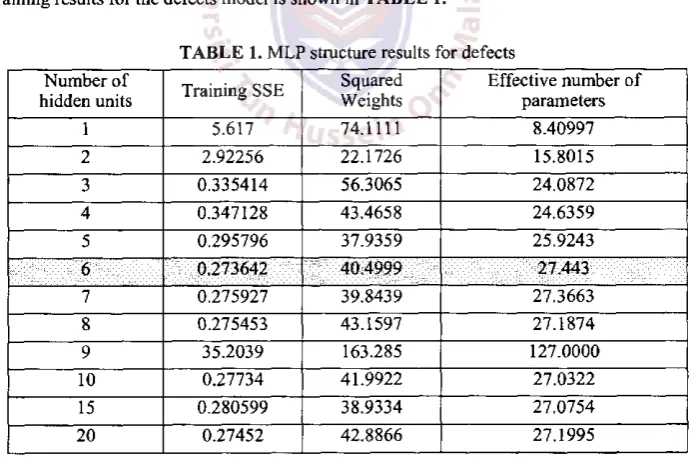
The M L P training was performed for 500 epochs (cycles) while the SSE performance function was used to evaluate the convergence of the M L P each time a hidden unit is added or removed. The optimal hidden layer size w a s found to b e 6 for both defects model. The M L P training results for the defects model is shown in T A B L E 1.

T A B L E 1. M L P structure results for defects

N u m b e r of

hidden units Training SSE

Squared Weights

Effective number of parameters 1 5.617 74.1111 8.40997 2 2.92256 22.1726 15.8015 3 0.335414 56.3065 24.0872 4 0.347128 43.4658 24.6359 5 0.295796 37.9359 25.9243 6 0.273642 40.4999 27.443 7 0.275927 39.8439 27.3663 8 0.275453 43.1597 27.1874 9 35.2039 163.285 127.0000 10 0.27734 41.9922 27.0322 15 0.280599 38.9334 27.0754 20 0.27452 42.8866 27.1995

N u m b e r u f D a f a u U s w i l h B h i d d e n u r i i l y

FIGURE 1. Modelling results for defects model with 12 variable

4.3 Feature selection using Particle Swarm Optimization (PSO)

The P S O was used to select the three best inputs to explain the input-output relationship of defects model. A ranking-based system was used to select the best features. Using this system, the value of each particle in the swarm represents the importance of each feature. During optimization, the three best-ranked features were used to train the M L P .

The objective of the PSO is to minimize the M S E fitting error between the actual output and the modelled output. If the features are discriminative, the generalization error should be small since the M L P approximation is close to the actual output. If the features are not discriminative, the model approximation should be poor (indicated by high M S E values).Three experiments were performed to:

o Determine the swarm (population) size required for P S O to converge.

o Determine the best combination of features to minimize production defects.

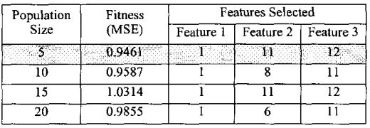
o Determine the best combination of features to minimize the machine adjustment time. The minimum population size required to converge is 5 for defects. Therefore, the population of 10 was chosen to sufficiently model both problems. Refer T A B L E 2.

T A B L E 2. Summary of results for population size for defects model

Population Fitness Features Selected Size (MSE) Feature 1 Feature 2 Feature 3

5 0.9461 1 11 12 10 0.9587 1 8 11 15 1.0314 1 11 12 20 0.9855 1 6 11

5. Conclusions

6.268. Meanwhile, population has 10 individuals convergence f r o m generation number 13 to 20 and best fitting on generation number 20 with best fitting value is 1.314.

s

-siiruhilwc WLF

n

l i

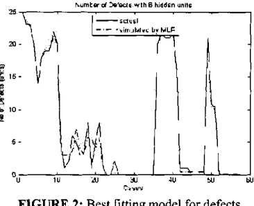
F I G U R E 2: Best fitting model for defects

Furthermore, G A gave improvement when population has 15 individuals convergence f r o m generation number 5 to 20 and best fitting on generation number 15 and 18 with best fitting value is 1.31. But population has 20 individuals gave the better on best fitting value to 1.309 on generation number 16.

The fitting value much better compare to others number of population.

The P S O was used to optimize the input values for the M L P . 6 units were used in the hidden layer. Both the defects and time models were tested. The objective of the P S O is to minimize either the number of defects or the manufacturing time. The fitness is calculated as number of defects or manufacturing time.

o Function \defects\ and \time\ were used as fitness functions,

o Both should yield 0 as best values.

Since the input should be within certain bounds, any value outside the range of [+1, -1] was clamped during preprocessing. The optimization w a s performed for 100 generations, with 10 particles for each population. Linearly decreasing inertia weight was used to ensure good convergence. The inertia weight starts with 1 and was decreased after each iterating until it reaches zero. The population test for the defects model is shown in T A B L E 3 and F I G U R E 3.

T A B L E 3. Optimization results (defects model) Particles Screw Pulling Line speed M S E

PSO Convergence with Population Size S

PSO Best Convergence with Population Size 5

Feature

F I G U R E 3. The defects optimization results using 5 particles

References

Eberhart, R.C and J.Kennedy (1995). A new optimizer using particle swarm theory. Proceeding of the Sixth Symposium on Micro Machine and Human Science. IEEE Service Center, Piscataway, NJ, 39-43.

H. Demuth and M. Beale.(2005). MATLAB Neural Network Toolbox v4 User's Guide. Natick, MA.: Mathworks Inc.

Hlupic, V. and Robinson, S. (1998). Business Process Modelling Using Discrete-event Simulation, Madeiras, D.J., Watson, E.F., Karson, J.S. and Manivannan, M.C. (eds.), Proceedings of the Winter Simulation Conference WSC'98, Washington D C , SCS, pp.

1363-1369.

Hlupic, V., de Vreede G. (2005). Business process modelling using discrete-event simulation: current opportunities and future challenges; invited keynote paper in the inaugural issue of International Journal of Simulation and Process Modelling, 1(1/2), pp. 72-8.

Kennedy, J. (1998). The Behavior of Particles. Evol. Progr. VII, 581-587.

M. Norgaard, O. Ravn, N. K. Poulsen, and L. K. Hansen.(2000). Neural networks for modelling and control of dynamic systems: A practitioner's handbook. London: Springer.

Y. Shi and R. C. Eberhart. (1998). A modified particle swarm optimizer, IEEE International Conf. on Evolutionary Computation. Anchorage, Alaska: IEEE Press, 69-73.

Shi, Y. H., Eberhart, R. C. (1998). Parameter Selection in Particle Swarm Optimization. The 7th Annual Conference on Evolutionary Programming, San Diego, USA.