Energy optimization in wireless sensor networks based on genetic algorithms

Energy

Op

t

im

iza

t

ion

in

W

ire

less

Sensor

Ne

tworks

Based

on

Gene

t

ic

A

lgor

i

thms

Ange

la

Rodr

iguez

-FUP Popayán, Colombia

[email protected] o

Pao

lo

Fa

lcar

in

School of Architecture, Computing and Engineering University of East

London London, UK [email protected]

Armando

Ordóñez

-FUP Popayán, Colombia

[email protected] o

Abstract—Wireless sensor is a consolidated technology with high potential in the Internet of Things. However, some open issues must be tackledin order toleverage the whole potential of this technology. One of the challengesis the energy consumption. Many algorithms have been proposed for saving energy. However these approaches use a mono-objective evaluation and the contradiction between optimization parameters values is not considered. Besides these approaches don’t offer a unique solution. This paper describes MOR4WSN an algorithm basedin NSGA-II for selecting the best sensor distribution as well as a mechanism for optimization of results. Experimental evaluation shows promising resultsin terms oflifetime maximization.

Keywords—wireless sensor networ ks; genetic algorithm; mult i-objective optimization

I. INTRODUCTION

Internet ofthings (IoT)is based onthe pervasive presence of objects or elements such as RFID (Radio frequency identification), sensors, mobile devices, etc. These elements interact with each other in orderto reach a common goal [1]. Among this wide set of objects, wireless sensor networks (WSN) play an important role as they allow to collect information from the context which is useful for decision making [1]. Due to advances in sensor technology, these sensors are becoming more and more powerful, economic and smaller. This situation hasleveraged deployment of high scale WSN with hierarchy or cluster based topology. One of the main challenges of IoT is energy optimization in each object [2].

Particularly, high scale WSN must afford challenges such as preservation of network longevity. This longevity is reachedin part withthe reduction of energy consumption due to the fact that sensor have limited energy sources which usually cannot be reloaded once the network is deployed in remote or difficult access areas. While WSN is in operation modethe higher energy consumptionis produced during data transmission due to the use of radiofrequency module [1]. Consequently, one of the key factors for optimization of battery lifetime is right selection of paths for information gathering;thelatter meansto selectthe best routingtopology according to WSN requirements. In this regard, there exist diverse factors that affect battery consumption during data

transmission such as: distance between sensors, network topology, among others. Consequently,this optimization may be seen as a multi objective optimization problem.

Previous approaches [3][4][5][6][7] have used bioinspired techniques such as ant colony optimization or evolutionary techniques like genetic algorithms for defining transmission routes in WSN. However, these works don’t consider multi objective optimizationthat allowstoinclude diverse factorsin the analysis. Besides these approaches don’t offer a unique solution to the optimization problem but a set of solutions. Previously [8] the evolutionary multi-objective algorithm NSGA-II was proposed for optimization of energy consumption in hierarchical WSN. Here, the experimental results of MOR4WSN (Multi-Objective Routing for WSN) algorithm based on NSGA-II are presented. This paper presents the modeling of hierarchical WSN in chromosomes forits use in MOR4 WSN; equallyit is presented design and implementation of objective functions for optimization of data gathering pathsin hierarchical networks. Experimental results are also presentedinthis paper.

The rest of this paper is organized as follows: Section 2 presents conceptual background, Section 3 describes the modelling of WSN in genetic algorithms, Section 4 presents the objective functions. Latter Section 5 showsthe evaluation of WSNlongevity byintroducing MOR4WSNinthe network. Section 6 describes the related work and finally section 7 details conclusions and future work.

II. BACKGROUND

A. Wireless Sensor Networks

WSN are composed of many sensor nodes known as source nodes which gather data from environment using a sensing module and communicate with other nodes through wirelesstechnologiesin orderto send datatothe central point known as base station or sink node.

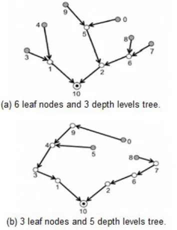
As WSN lacks of physical infrastructure, so these WSN can adopt different topologies according to the domain. The most common topology for high scale networks like IoT networks used for city or parks monitoring is the tree or hierarchical topology. Fig. 1 shows a tree WSN rooted with the base station whilethe rest ofthe nodes are data sources.

Fig. 1. WSN with hierarchicaltopology

Next, terminology associated with hierarchical topologies is presented.

Source node: node that picks up information from environment and send this information to the base station. Leaf node: nodethat does not have childreninthetree,thatis, the one that does not receive data from other nodes to be transmittedtothe base station. Tree depth: maximum amount of hops between nodesthat must be done by a source node for reaching a base station. Routing node: nodethat receives data from one or many nodes and retransmit them to other node addingits data. WSN routing: needed mechanismsto carry out data transmission from source to destination [9]. Network longevity:time between start-up of WSN until the moment that one node or a percentage of them is unable of sending datato base station.

It has been proved that efficient data routing is crucial in decreasing energy consumption [3]. In this vein, reduction of energy consumption directly affect networklongevity.

B. Genetic algorithms

Genetic algorithms start from a set of possible solutions randomly generated (initial population) called chromosomes (or individuals) that consist of a set of gens with the same length (see Fig. 2). Genetic algorithms include a fitness functionthat assigns a value to each individual based on the proximitytothe optimal solution. In orderto get closertothe optimal solutions, diverse genetic operators are appliedtothe initial population. Some of these operators are: selection allowsto create offspring fromthe process of crosover oftwo parent chromosomes. Mutation alter genetically oneindividual information in order to improve the criteria to be optimized [10]. Fitness functions are applied to all populations to determinethe proximityto optimal solution.

Fig. 2. Chromosome with 6 gens

C. Multi- objective evolutionary algorithms

In contrast to simple genetic algorithms, multi-objective techniques aims to find solutions to problems that require optimization of several objectives (which may be opposed to each other) atthe sametime. Multi objective genetic algorithm (MOGA) modifiesthe way of calculatingindividual fitness,to do so, a set of objective functions are required.

Due to multi objective nature, MOGA does not find an optimal solution, but a set of solutions known as Pareto front (or not dominated set). Pareto front includes best solutions considering all objectives under analysis. Some examples of MOGA are: Vector Evaluated Genetic Algorithm (VEGA), niched Pareto genetic algorithm (NPGA), Non-dominated Sorting Genetic Algorithm (NSGA). These algorithms have a computational complexity of 0(mN3_{), where m is the number}

of objectives and N is the size of the population. In order to get a lower complexity it is possible to reduce the search spaces by applying two concepts: elitism and diversity preservation. This latter is the foundation of NSGA II (Fast Elitist Non Dominated Sorting Genetic Algorithm) [11], which is an evolution of NSGA. NSGA II maintains diversity between solutions by incorporating two parameters: sharing and crowding distance. NSGA II got a reduction of complexity to 0(mN2_{), further details about NSGA II can be}

foundin [12] and [13].

III.WSNMODELING

A. Networkfeatures

Some common features of WSN deployed in huge extension areas are: distance between nodes can reach 100 meters.ii) Sensing and data gatheringis periodic.iii) Network longevity must reach several months.iv) Battery rechargingis difficult due to difficult access. v) Network topology is commonly hierarchical or cluster based.

B. Representation of Solutions

During WSN operation, it can happen that some routing nodes receive and retransmit packets from other nodes, thereby discharging batteries quickly. That is why it is important to keep the equilibrium in energy consumption between nodes by an equitable distribution of data packets to be processed, received and retransmitted. This equilibrium is known asload balance [14].

Parameters of tree topologies that most directly impact WSN routing are number of leaf nodes and tree depth [9]. The lower value of these parameters, the longer the network longevity. Based on the above, the objectives of the present approach to obtain optimal data transmission paths are: i) to decreasethe number ofleaf nodes andii)to decrease depth of the tree. Fig 3 shows an example of network in which objectives (i) and (ii) are contradictory. Therefore NSGA II could be appliedin such a case.

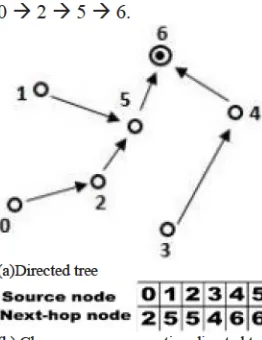
MOR4WSN adopts hierarchical WSN model in chromosomes from[3][4][5][6][7]. Let N bethetotal of nodes in a given WSN, in Fig. 4 the chromosome represents a routingtree where each nodeislabeled with aninteger from 0 to N. In Fig 4bthe gen valuein position 0is 2indicatingthat node 0 selects node 2totransmitits data, node 2transmitsto node 5,the valuein 5is 6indicatingthatthe next nodeis base station and therefore the full gathering path from node 0 is expressed asthe path

0 2 5 6.

(a)Directedtree

(b) Chromosome representing directedtree. Fig. 4. Routing solutionin a WSN

IV.OBJECTIVEFUNCTIONS INMOR4WSN

As mentioned before, monitoring tree networks reach greater longevity as long as leaf nodes and depth are minimized [9]; Fig. 3 shows how difficultisto get a network disposition that optimizes both parameters. In order to understand objective functions,itis necessarytointroducethe concept of Pareto Dominance shown in Fig 5. Pareto front represents the set of solutions considering all objectives to optimize [15]. In the example, a solution a ‘dominates’ to b providedthat: a won’t be worstthat b in all objectives, anda is strictly betterthatb atleastin one objective. Thusthe set of solutions not dominated by other solutions makes up non dominated front (or Pareto non dominated solutions) [11]. In Fig. 5 these solutions are represented by points 3 and 5, whereas functions f1 andf2 represent problem objectives.

Non dominated solutions set (optimized chromosomes) are equally good anditis hardto determine which one ofthemis betterthan others, except when decision making experts have defined preferences a priori [15]. However the cardinality of this set in M, been M the size of the population. In this context, NSGA II results for a network with 100 nodes contains 100 chromosomes (optimizedtrees) each one ofthem

with a size of 100, and for the network operationit is needed to select only one solution that represents the network disposition. As this process is hard to do manually, our approach includes a mechanism that compares chromosomes by pairsin orderto selectthe best solution automatically;this approachis based on binaryindexes andis widely describedin [16].

Fig. 5. Pareto front and dominance

Due to its evolutionary nature, in NSGA II any potential solution is codified as a set of characters containing all the needed information for calculating objectives functions (see Fig. 4). These objectives functions are applied to each chromosometo classifythem accordingits fitness value.

As aforementioned in section 3, MOR4WSN works under two objective functions: f1 to decrease the number of leaf

nodes, and f2 to decrease the depth of the routing tree. By

analyzing Fig. 4a.itis clear that the example directed acyclic graph has three leaf nodes labeled as 0, 1 and 3. In Fig. 4b. one can beinfer that leaf nodes identifiers does not appear in the allele’s row represented bythe string ofintegers. Theleaf nodesin Fig. 4a are preciselythosethat don’t have a place in the allele ubication of Fig 4b.

Onceleaf nodes areidentified inthe chromosome,it must be followedthe multi hop path between nodes by which each leaf node sends data to base station. Thus, node 0 has a transmissionlink 0 2 5 6; going onthe chromosome for identifying the path for node 1 we get: 1 5 6 and finally for node 3, the pathis 3 4 6. The longer path is the one of node 0 with a total of 3 hops between nodes, whereas leaf nodes 1 and 3 have paths with length 2. Consequently, tree depth in this example is 3. NSGA-II code includes a method which allows to define the number of objectives of each problem as well astheimplementation, our approach is based in the algorithm described in [13]. In MOR4WSN functions f1 andf2 areimplemented as shownin Fig. 6, where vector obj represents the set of objective functions. Finally, each functionis multiplied by -1 duetothe fact that NSGA II aims for minimizing values of each function.

#ifdef leafsHops

void test_problem (double *xreal, double *xbin, int **gene, double *obj, double *constr)

leaf=(int *) malloc(sizeof(int)*(nreal+1));

/* vector initializacion, asssuming that all nodes are leaf excepting the base station */

for(i=0;i<nreal;i++){ leaf[i]=1; }

leaf[nreal]=0;

/* Counting non leaf nodes.*/ for(i=0;i<nreal;i++){

if(leaf[(int)xreal[i]]==1){ leaf[(int)xreal[i]]=0; noLeaf++;

} }

/*Calculus of the number of leafs.*/ leafs=nreal-noLeaf;

int nextHop=0, hops=0, maxHops=0;

/*Going over the leaf vector to count the hops done by each leaf*/

for(i=0;i<nreal;i++){ hops=0;

if(leaf[i]==1){ nextHop=i; do{

nextHop=xreal[nextHop]; hops++;

}while(nextHop!=nreal); if(hops>maxHops){ /* Maxmimun number of hops of a leaf node */

maxHops=hops; }

} }

obj[0]=(-1)leafs; obj[1]=(-1)maxHops; }

#endif

Fig. 6. Implementation of objective functionsin MOR4WSN

V. EVALUATION

MOR4WSN finds routing structures optimized according to f1 and f2, in such a way that these structures preserve

longevity (in terms of sensing rounds) in the WSN. For evaluation purposes MOR4WSN was compared with the routingtechnique used by ZigBee for hierarchicaltopologies: Tree Routing (TR). No other multi-objective approach for data routingin WSN where foundintheliterature, sothat choosing a standard algorithm as Tree Routing is an appropriate wayto get comparative results in order to evaluate how a mult i-objective evolutionary alternative contributes to network longevity.

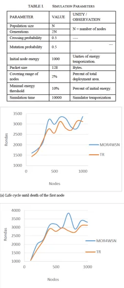
During simulation execution the following data for different network dimensions weretaken:i) Lifetime untilthe first node dies. ii) Life time until 10% of nodes die. iii) Life time until 30% of nodes die. Table I lists values adjusted to simulation parameters, assuming homogeneous networks,that means all nodes having the same initial energy level and its covering range beingthe same. Results of comparativetest are shownin Figs. 7a, 7b y 7c.

As showninthe evaluation results of Fig. 7,inclusion of a multi-objective alternative for selection of tree topology increases network longevity even up to 23%. In the three evaluated cases, albeit fluctuations in curves showing the

number of rounds, MOR4WSN exceeds in 85% of measures the longevity of standard algorithm Tree Routing whose only criteriais number of hopsto base station [9]. Equally, Fig. 7 shows that advantages in life cycle of MOR4WSN are independent ofthe number of nodesinthe network.

TABLE I. SIMULATIONPARAMETERS

PARAMETER VALUE UNITY_OBSERVATION /

Population size N

N = number of nodes Generations 2N

Crossing probability 0.5

----Mutation probability 0.5 _-

---Initial node energy 1000 _temporUnities of_iza ene_tionrgy_.

Packet size 128 Bytes. Covering range of

nodes 2% Pedeprcenloyment oftot area.tal Minimal energy

threshold 10% Percent ofinitial energy. Simulationtime 10000 Simulatortemporization

(a) Life cycle until death ofthe first node

(b) Life cycle until death of 10% of nodes

1000 1500 2000 2500 3000 3500

0 500 1000

Ro

nd

as

Nodes

MOR4WSN TR

1000 1500 2000 2500 3000 3500 4000

0 500 1000

Ro

nd

as

Nodos

(c) Life cycle until death of 30% of nodes Fig. 7. Lifetime of WSN

VI. RELATEDWORKS

Many approaches [3][4][5][6] have used genetic algorithms to combine routing parameters in a WSN and to define gathering routes that optimize energy consumption. These approaches are based on simple genetic algorithms (mono-objective) combining diverse variables in a single function called fitness function (see table II). Fitness function does not consider the contradiction of optimizing many variables concurrently. Thisis duetothe factthatthe resultis obtained from the weighting sum where weights have been defined a priori by experts. Even though, some approaches [3][4][5][6] that use routing trees, they don’t consider some variables associated withthese hierarchicaltopologies such as leaf nodes andits depth.

TABLE II. RELATED WORK

Fitness function

[3] _paDis_thtance_{, dis} be_tancetween _from node _curren pairs_{t node}, ave_torage_the ene _basergy _s of_tatthe_ion. [4] Total distance covered by nodesin each round.

[5]

Distance between nodes emitter and receptor, residual energy of both. Descendants are compared withtheir parents accordingtothe energylevelin orderto reviewif new chromosomes are better. [6] _transmResidua_issl ene_ionrgy _and of _recep curren_tiont node anditsload of

VII. CONCLUSIONS

Energy optimization in WSN can be seen as a mult i-objective problem. The presented approach showsthe creation of objective functions that allowto optimize different criteria at the same time. MOR4WSN allows finding tree topology that exceedsthelongevity of standard algorithmTree Routing used by ZigBee. Equally MOR4WSN is independent of the number of nodesinthe network.

Adaptation of NSGA-II allows to conclude that genetic operator(crossing, mutation, andinitial population generation) must be tuned carefully to WSN conditions. For example a chromosome like the one shown in Fig. 4 must always represent an acyclic structure, otherwise it would be inadmissiblein Pareto non dominated set. As future work,itis envisaged to test MOR4WSN in IoT networks with different devices and features. Equally we planto carry out calculus of tree depth using hops average of allleaf nodesinstead of using justthe deepest branchlength value.

REFERENCES

[1] Atzori, Luigi, Antonio Iera, and Giacomo Morabito. "The internet of things: A survey." Computer networks 54.15 (2010): 2787-2805. [2] D. Giusto, A. Iera, G. Morabito, L. Atzori (Eds.), The Internet of Things,

Springer, 2010. ISBN: 978-1-4419-1673-0.

[3] A. Bari, S. Wazed, A. Jaekel, and S. Bandyopadhyay, “A genetic algorithm based approach for energy efficient routing in two-tiered sensor networks,” Ad Hoc Netw., vol. 7, no. 4, pp. 665–676, Jun. 2009. [4] A. Chakraborty, S. Kumar, and M. Kanti, “A genetic Algorithm Inspired Routing Protocol for Wireless Sensor Networks”, International Journal of ComputationalIntelligence Theory and Practice, vol. 6 no. 1, 2011. [5] S. K. Gupta, P. Kuila, and P. K. Jana, “GAR: An energy efficient

ga-based routing for wireless sensor networks,” in Distributed Computing and Internet Technology, Springer, 2013, pp. 267–277.

[6] O. Islam, S. Hussain, and H. Zhang, “Genetic algorithm for data aggregationtreesin wireless sensor networks,” 2007.

[7] I. Apetroaei, I.-A. Oprea, B.-E. Proca, and L. Gheorghe, “Genetic algorithms applied in routing protocols for wireless sensor networks,” 2011, pp. 1–6.

[8] A. M. Rodríguez, y J. C. Corrales, “Técnica evolutiva para enrutar datos de una red de sensoresinalámbricos en el contexto dela agricultura de precisión”, VII Congreso Iberoamericano de Telemática: cita2015, Popayán – Colombia. En evaluación.

[9] A. M. Ortiz Torres, "Técnicas de enrutamientointeligente para redes de sensores inalámbricos". Tesis doctoral. Universidad de Castilla La Mancha. Albacete – España, 2011.

[10] López, J. “Optimización Multi-objetivo Aplicaciones a problemas del mundo real.” Tesis doctoral. Facultad de Informática Universidad Nacional dela Plata, (2013).

[11] K. Deb, S. Agrawal, A. Pratap, and T. Meyarivan, “A fast elitist non-dominated sorting genetic algorithm for multi-objective optimization: NSGA-II,” Lect. Notes Comput. Sci., vol. 1917, pp. 849–858, 2000. [12] León Javier, A. “Diseño eimplementación en hardware de un algoritmo

bioinspirado.”, Tesis de Maestría. Instituto Politécnico Nacional. México D.F., (2009).

[13] K. Deb, A. Pratap, S. Agarwal, and T. Meyarivan, “A fast and elitist multiobjective genetic algorithm: NSGA-II,” Evol. Comput. IEEE Trans. On, vol. 6, no. 2, pp. 182–197, 2002.

[14] X. Cui and Z. Liu, “BCEE: a balanced-clustering, energy-efficient hierarchical routing protocolin wireless sensor networks,” 2009, pp. 26– 30.

[15] I. Cabezas and M. Trujillo, “A Method for Reducing the Cardinality of the Pareto Front,” in Progress in Pattern Recognition, Image Analysis, Computer Vision, and Applications, Springer, 2012, pp. 829–836. [16] A. Rodríguez, A. Ordóñez, A. Ordóñez, “Energy consumption