Semiparametric estimation of diffusion models with applications in finance

w ith A pplications in Finance

D e n n is K r is te n se n

P h .D . T hesis D e p a rtm e n t of E conom ics,

L o ndon School of E conom ics a n d P o litica l Science

UMI Number: U190353

All rights reserved

INFORMATION TO ALL USERS

The quality of this reproduction is dependent upon the quality of the copy submitted. In the unlikely event that the author did not send a complete manuscript

and there are missing pages, th ese will be noted. Also, if material had to be removed, a note will indicate the deletion.

Dissertation Publishing

UMI U190353

Published by ProQuest LLC 2014. Copyright in the Dissertation held by the Author. Microform Edition © ProQuest LLC.

All rights reserved. This work is protected against unauthorized copying under Title 17, United States Code.

ProQuest LLC

789 East Eisenhower Parkway P.O. Box 1346

F

Abstract

1 Introdu ction 7

2 E stim ation in Diffusion M odels 11

2.1 In tro d u c tio n ... 11

2.2 Diffusion P r o c e s s e s ... 12

2.3 Estim ation in Scalar Diffusion M o d e l s ... 14

2.3.1 The Param etric M o d e l... 14

2.3.2 The N onparam etric M o d e l... 16

2.3.3 Two Classes of Semiparametric Models ... 20

2.4 Conclusion ...21

3 Term Structure M odelling w ith Diffusions 22 3.1 In tro d u c tio n ...22

3.2 The Arbitrage-Free Term S tr u c tu r e ... 22

3.3 The M ulti-Factor M o d e l ...25

3.4 The H eath-Jarrow -M orton M o d e l...27

3.5 Conclusion ... 28

4 E stim ation in T w o C lasses o f Sem iparam etric Diffusion M odels 29 4.1 In tro d u c tio n ...29

4.2 Framework ...32

4.3 The N onparam etric E s tim a to r... 37

4.4 The Semiparametric E s t i m a t o r ...42

4.4.1 Class 1 43 4.4.2 Class 2 ... 49

4.5 Semiparametric E ffic ie n c y ...51

4.6 Im p le m e n ta tio n ... 53

4.7 A Simulation Study ... 54

Contents 2

4.A P r o o f s ... 58

4.B L e m m a s ... 64

4.B.1 Class 1 67

4.B.2 Class 2 ... 84

4.B.3 Auxiliary L e m m a s ...89

5 E stim ation o f Partial D ifferential E quations 104 5.1 In tro d u c tio n ...104

5.2 Linear Parabolic P artial Differential E q u a t i o n s ...107

5.2.1 Applications in F i n a n c e ... I l l 5.2.2 Estim ation of Diffusion M o d e ls ... 115

5.3 Estim ation of P artial Differential E q u a t io n s ...116

5.3.1 A Param etric E s ti m a t o r ... 120

5.3.2 A Semiparametric E s t i m a t o r ... 123

5.3.3 A Nonparam etric E s tim a to r ...126

5.4 A p p licatio n s...129

5.5 Conclusion ... 132

5.A P r o o f s ...133

5.B Auxiliary L e m m a s ...142

5.B.1 The Semiparametric E s t i m a t o r ... 147

5.B.2 The Nonparam etric E stim ator ... 149

6 A Sem iparam etric Single-Factor M odel o f th e Term Structure 155 6.1 In tro d u c tio n ...155

6.2 Single-Factor Term S tructure M o d e ls ... 157

6.3 Estim ation of the Risk P r e m i u m ...159

6.4 The D a t a ... 161

6.5 Empirical R e s u lts ... 165

6.5.1 Estim ation of the Single-Factor M o d e l ... 165

6.5.2 Implied Bond and Derivative Prices ... 172

6.6 Conclusion ... 174

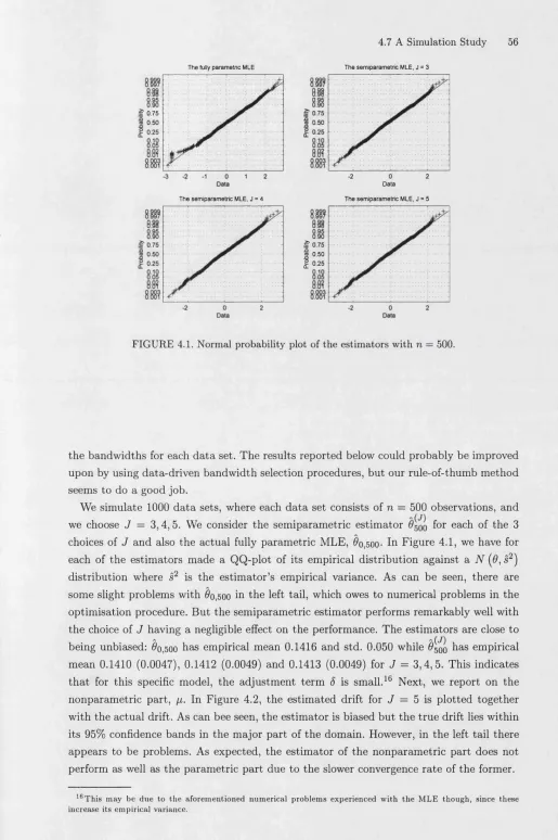
4.1 Normal probability plot of the estim ators w ith n = 500... 56

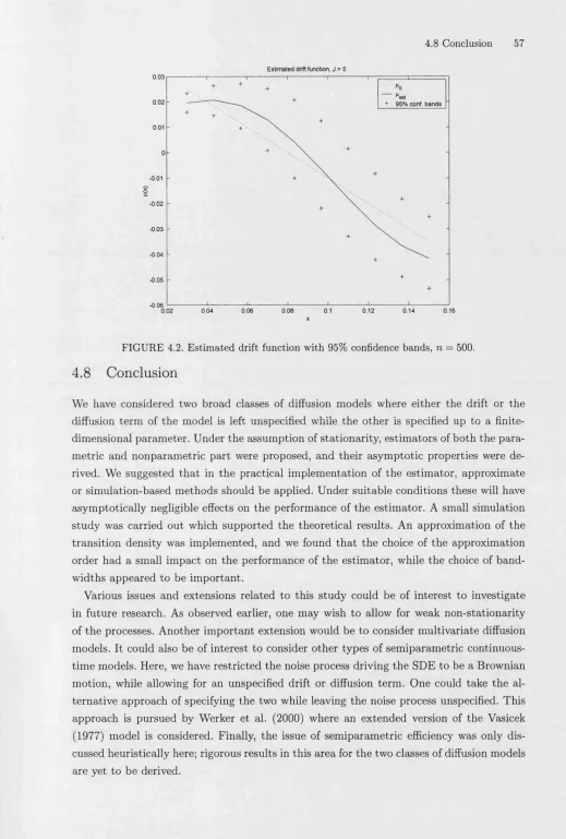
4.2 Estim ated drift function w ith 95% confidence bands, n = 500... 57

6.1 The Eurodollar spot rate in levels, 1973-1995... 164

6.2 The Eurodollar spot rate in differences, 1973-1995... 164

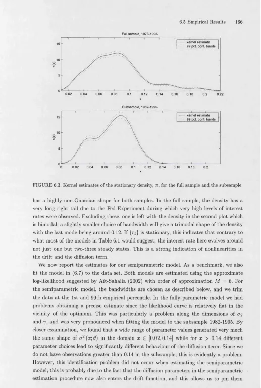
6.3 Kernel estim ates of the stationary density, 7r, for the full sample and th e subsam ple... 166

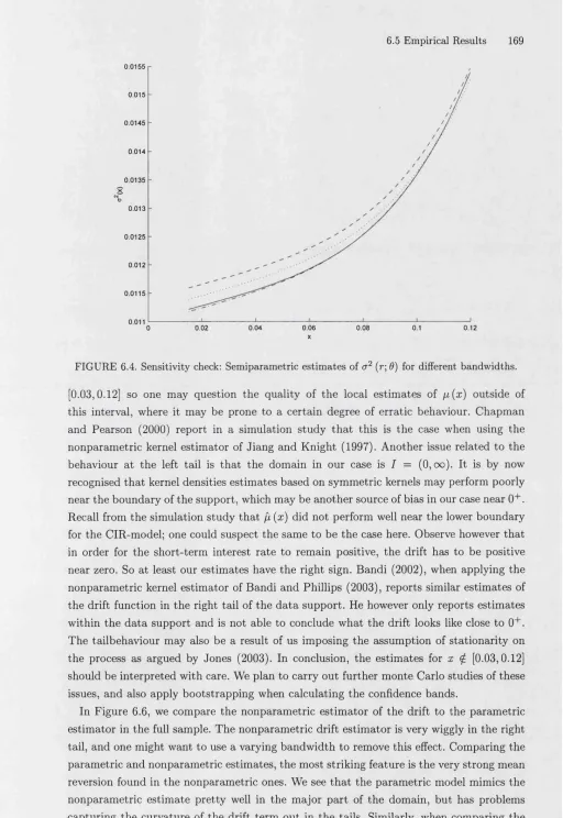
6.4 Sensitivity check: Semiparametric estim ates of a 2 (r; 9) for different band-w idths... 169

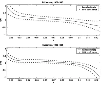
6.5 N onparam etric estim ate of fi w ith 95% confidence bands...170

6.6 Comparison of nonparam etric and param etric estim ate of /z for th e full sample, 1973-1995... 171

List of Tables

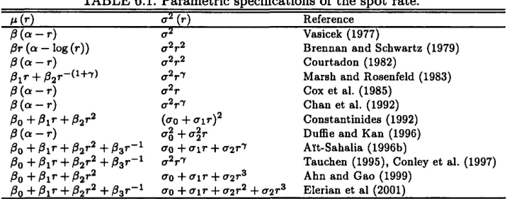
6.1 Param etric specifications of th e spot ra te ... 159

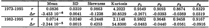
6.2 D ata descriptives...165

6.3 U nit root test results...165

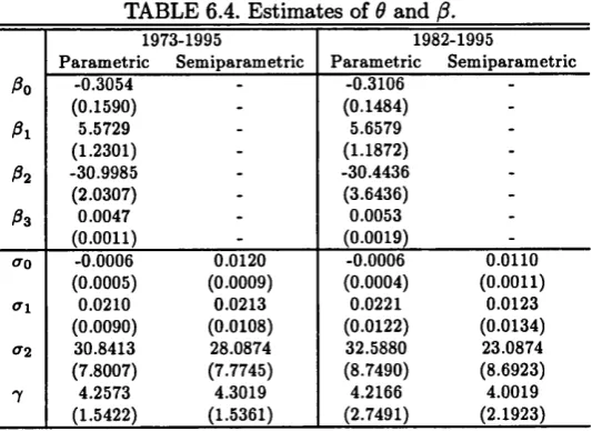
6.4 Estim ates of 9 and ft... 167

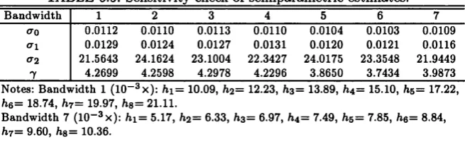
6.5 Sensitivity check of semiparametric estim ates...168

6.6 E stim ate of the market price of risk, A... 173

This thesis has been subm itted to the University of London in partial fulfillment of the requirements for the Ph.D . degree in Economics a t the London School of Economics and Political Sciences (LSE).

Throughout my studies at the LSE, I have received invaluable encouragement and sup­ p o rt from my supervisor, Oliver Linton, for which I am very grateful. Oliver has been a very inspiring guide into th e world of non- and sem iparam etric econometrics. Anders Rahbek, Richard Blundell, and Xiaohong Chen have also been a great support during my postgraduate studies. M atthias Hagmann, Antonio Mele, Peter Robinson have read various parts of the m anuscript. I am grateful for their comments and suggestions.

I would like to thank fellow students and researchers a t the D epartm ent of Economics and the Financial M arkets Group (FMG) a t the LSE for making my four years there such a great experience. P a rt of the work presented here was done while I was visiting th e Centre for Applied Microeconometrics (CAM) and the D epartm ent of Statistics and Operations Research (ASOR) a t University of Copenhagen, and the D epartm ent of Economics a t Yale University. Thanks to everyone a t the respective places for making these enjoyable visits. Financial support by th e Danish Research Agency, the FMG and the D epartm ent of Economics a t the LSE is gratefully acknowledged.

Introduction

Continuous tim e stochastic processes are widely used in dynamic models in economics and finance to describe phenom ena evolving random ly over time, see e.g. Bergstrom (1990) and Duffie (1996). In finance, these have been used in m athem atical models in areas as diverse as portfolio management, term stru cture modelling and asset pricing theory. In asset pricing theory these have been extensively used in th e derivation of pricing formulae. Since the now famous option pricing models by Black and Scholes (1973) and M erton (1973, 1976), diffusion processes have played a vital role in this p art of the finance literature. The main reason for the popularity of diffusion processes is th a t they enjoy a number of attractive properties which facilitates the theoretical analysis of th e models. In particular, one has at one’s disposal the powerful tools found in stochastic calculus. W ith these tools, assuming th a t the fundam ental asset prices follows a diffusion process, one can derive closed form expressions of a contingent claim using hedging and no-arbitrage arguments.

These continuous-time models are often calibrated and tested using historical data. For a review of th e empirical work using continuous-tim e models in finance, we refer to Sun- daresan (2000). T he im plem entation of th e models very often involves an estim ation step where the model is calibrated to the d a ta set at hand. Most frequently, the economic variables of interest are observed a t discrete points in time, e.g. daily, weekly or monthly observations, so-called discrete observations. As a first step, one needs to choose a statis­ tical model for the diffusion process in question. The second step will then involve finding an appropriate estim ator of the (possible infinite-dimensional) unknown param eters ap­ pearing in the model. The second step can become very involved due to th e fact th a t analytical expressions of the conditional density, moments etc. of the discretely sampled process are not available.

is as follows:

C h a p t e r 2: E s tim a tio n in D iffu sio n M o d e ls . We first introduce th e class of diffusion processes and present some of basic properties of these, and then gives an overview of the literature on the estim ation of diffusion models. We distinguish between three different sampling schemes (continuous record, discrete sample w ith shrinking tim e distance, and discrete sample with fixed tim e distance), and three types of models (param etric, semi­ param etric and nonparam etric). We pay particular attention to non- and semiparametric estim ation m ethods which have proliferated in recent years. As p art of the chapter, we therefore give a brief introduction to kernel- and series m ethods which are th e two main approaches used in non- and sem iparam etric econometrics. The main conclusion of the chapter is th a t while for the two first sampling schemes estim ators are derived in a fairly straightforward m anner, the th ird one is more problematic.

C h a p t e r 3: T e rm S t r u c t u r e M o d e llin g w ith D iffu sio n s. One particular area where diffusion processes are widely used is in th e modelling of the term structu re of interest rates. In this chapter, we give an overview of the most im portant models proposed in the literature, and the implications for bond and interest rate derivative pricing are discussed. T he m ain emphasis is on the class of single-factor models, a simple yet flexible class of interest rate models. Most of th e proposed specifications in the single-factor case are fully param etric models. None of these have proved to be very good a t describing th e observed interest rates. In C hapter 4 we therefore propose two classes of sem iparam etric models which can be used to model the term structure, and in C hapter 5 dem onstrate w hat con­ sequences the use of fitted versions of these will have for implied bond and interest rate derivative prices.

C h a p t e r 4: E s tim a tio n in T w o C la sse s o f S e m ip a r a m e tr ic D iffu sio n M o d e ls . We here set up two general classes of sem iparam etric scalar diffusion models, and propose an estim ator of both its nonparam etric and param etric p art given discrete observations w ith fixed sampling distance. The estim ator of th e param etric p art is a maximum-likelihood- type, while the nonparam etric p art is estim ated using kernel m ethods We derive the asym ptotic distribution of th e estim ator under regularity conditions. This is followed by a discussion of the issue of semiparametric efficiency. We propose a 1-step Newton-Raphson estim ator which should reach the effiency bound. A small simulation study examines the quality of the estim ator in finite sample.

1. Introduction 9

param etric ones. In all three cases, th e asym ptotic distribution of th e solution is derived. In particular, we consider the estim ator proposed in C hapter 4. We dem onstrate how these results can be applied in th e presented examples from the asset pricing theory.

C h a p t e r 6 : A S e m ip a r a m e tr ic S in g le -F a c to r M o d e l o f th e T e r m S tr u c t u r e . This chapter is an empirical study where th e results of C hapter 4 and 5 are employed in the modelling and estim ation of a sem iparam etric single-factor interest ra te model. We com­ pare th e fitted sem iparam etric model w ith standard fully param etric ones: F irst directly, by testing the fully param etric model against the sem iparam etric one. Secondly, we look at how much th e bond prices predicted by the com peting models differ; this yields an alternative measure of the performance of the models. The fitted sem iparam etric model picks up nonlinearities which the fully param etric model cannot capture. This leads to a rejection of th e param etric model in favour of the sem iparam etric model in the direct comparison of the two fitted models. Moreover, the calculated bond prices implied by the two com peting models are shown to be significantly different.

T he chapters can be read independently of each other. This means however th a t some definitions, results etc. are repeated in th e different chapters. I have tried to m aintain the same notation throughout the thesis, bu t there may be some slight differences; this should hopefully not cause any confusion. Throughout the thesis, the following notation will be used:

R 9 - th e space of ^-dimensional real vectors

R 9Xp - the space of q x p dimensional real matrices

At - th e transpose of any m atrix A

int (A)- the interior of any set A C - a generic constant

E [•] - th e expectations operator var (•) - the variance operator cov (•, •) - the covariance operator

1a (•) - the indicator function for any set A

~ - ’is distributed as’

—>p and —>d- convergence in probability and distribution respectively

{X*} - short for {Xf|0 < t < T ] for some 0 < T < +oo. The value of T will in most cases be evident from the context; we shall specify T when deemed necessary.

{xn} - short for {xn |l < n < N } for some 1 < N < +oo. T he value of N will in most cases be evident from the context; we shall specify N when deemed necessary.

For / : R x 0 h R, 0 C Rd, we shall use d lJ ef (x ; 9) to denote d*d*f (x; 9) / d %xd^9. In some cases, we shall write /W (x;9) for d * /( x ;0 ) , / (x; 9) for d $ f (x\ 9), and / ‘ (x; 9) for

a$f(x-,e).

For / : R d x 0 i—> R, we shall use d £ f (x; 9) to denote dn • • ■ d tdf (x; 9) / d n x i • • • d idXd for any d-tuple of non-negative integers, a = ( z i,..., id).

Estimation in Diffusion Models

2.1

Introduction

We here give a brief introduction to diffusion processes, present some of their basic prop­ erties, and then give a review of the literature on estim ation of diffusion models. This literature spans a period of over th irty years and covers a wide range of different topics. We shall in th e following try to give an overview of the m ain results w ith emphasis on non- and sem iparam etric estim ation of discretely observed diffusions. We have chosen to classify the results presented here along two dimensions: Along the first, we have the type of model and along the second, the type of sampling scheme. We shall focus solely on time-homogenous, stationary scalar diffusions. No formal proofs are given, b u t references to the relevant studies are given.

The above problems associated w ith the estim ation given discrete observations can be circumvented by assuming th a t the tim e distance between observations go to zero asymptotically. In this setting, th e standard strategy is first to define an estim ator of the continuously sampled process, and check th a t this has th e desired properties. Then one can normally construct a suitably discretised version of this which can be used for a discrete sample. The discretisation error due to th e discrete approxim ation will vanish asym ptotically if the tim e distance between observations goes to zero sufficiently fast. This approach will unfortunately lead to an asym ptotic bias when one assumes a fixed positive tim e distance between observations.

The chapter is organised as follows: First, in Section 2, we introduce th e class of diffusion processes and some of its im portant properties. In Section 3, we then tu rn to th e question of estim ation where we first define the d ata generating process, and th e three sampling schemes in question: Section 3.1 deals w ith the fully param etric case, Section 3.2 w ith the nonparam etric model, while the sem iparam etric case is treated in Section 3.3. For each type of model, we differentiate between the three sampling schemes. Finally, we conclude in Section 4.

2.2 Diffusion Processes

We consider a process { X t} taking values in R9. The process is assumed to solve a stochastic differential equation (SDE) of the form

d X t = fi (t, X t ) dt + a (t, X t) dW t (2.1)

defined on a filtered probability space P ) w ith associated filtration {Ft}- T he above formulae should be read as

X t = X o +

f

Jo Jo

where {W t} is a ^-dimensional standard Brownian motion. T he function /x : [0, oo) x R ? h

R 9 is normally called the drift term while a 2 : [0, oo) x R9 i—► R 9*9 is called th e diffusion term. The drift and diffusion term can be interpreted as th e instantaneous conditional mean and variance respectively,

= Um ■ZJpft+A - X t \Xt = x] ,

<t2 («,x) = ^ i m £ [ ( X , + A - X () ( X t+ A - X () '1X t = x ].

F urther introduction to and treatm ent of stochastic differential equations and diffusions can be found in, am ongst others, K arlin and Taylor (1981), K aratzas and Shreve (1991),

Rogers and Williams (1994, 1996). We shall assume th a t a unique weak solution to (2.1)

2.2 Diffusion Processes 13

of th e following, we shall only be concerned w ith time-homogenous SDE’s,

d X t = p ( X t ) dt + tJ ( X t ) dW u (2.2)

where the drift and diffusion term do not depend directly on the tim e param eter t.

T he conditional distribution of X t+& conditional on X t is given by the transition density

p (t + A, -\t, x). For the time-homogeneous SDE, p satisfies p (t + A, -|£, x) = p& (*|x). Only in a few special cases is it possible to obtain an analytical expression of p. U nder suitable conditions, cf. K aratzas and Shreve (1991, Section 5.5) and Meyn and Tweedie (1993), there exists an invariant density 7r for the tim e homogenous model.

In the univariate case (q = 1), one can furtherm ore derive an expression for 7r,

7r (x) = [M a 2 (x) s (x)] 1 (2.3)

where s (x ) = exp[—2 f*mp ( y ) /c r 2 (y)dy\ is the scale function for some x* E I, where

I = (Z,r), —oo < I < r < +oo, denotes the domain of the process, and M > 0 is a normalising factor. If the process is initialised w ith Xq ~ 7r, we obtain a stationary and ergodic solution to (2.2). The distribution of the stationary solution {Xt} is denoted Pn.

Observe th a t th e relation (2.3) can be inverted to express p (cr2) in term s of 7r and a 2 (p):

(2-4)

a2 W = V P_{n (x ) Jl}a I P ^ dy' (2-5)

The class of diffusion processes proves to be closed to sm ooth transform ations. For any twice differentiable function / : R 9 R, the process Yt = f (Xt) solves

dYt = L t f ( X t ) dt + Qxf ( X t ) a (£, X t ) dW t (2.6) where Lt is the so-called infinitesimal generator defined by

T \ \ d f (x) 1 o \ d 2f (x )

Ltf

>

i=l i,j=1 J

see K aratzas and Shreve (1991, p. 281). This is the celebrated l t d ’s Lemma. Taking con­ ditional expectations in (2.6), one obtain for t < T,

E [ / ( X T ) ] X t = x\ = [ L , E [ / ( X . ) \X ,= *x]ds.

Differentiating w .r.t. t on bo th sides of the above equality, we obtain th a t th e function

A formal proof of the above can be found in K aratzas and Shreve (1991, Theorem 5.7.6). This is th e simplest version of the Feynman-Kac formula.

2.3 Estim ation in Scalar Diffusion Models

We shall in th e following discuss th e estim ation of the drift and diffusion function in a param etric, nonparam etric and sem iparam etric framework. Throughout this section, the d a ta generating process {X t} is assumed to be stationary and solve the univariate SDE

d X t = fi0 ( X t ) dt + <J0 ( X t ) dWt, (2.8) where {W t} is univariate. We shall not discuss the estim ation of m ultivariate or nonsta- tionary models. Estim ation m ethods for m ultivariate param etric diffusion models can be found in e.g. Al't-Sahalia (2003), Bibby and S0rensen (1995), Duffie and Singleton (1993), and Broze, Scaillet and Zakaian (1998). Bandi and Moloche (2001) and Chen, Hansen and Scheinkman (2000b) consider nonparam etric kernel and sieve estim ators respectively for m ultivariate processes, the former allowing for nonstationarity. Al’t-Sahalia (2002) gives a general result for the param etric MLE of nonstationary scalar diffusions. Bandi and Phillips (2003) and Nicolau (2004) develop kernel estim ators for nonstationary scalar dif­ fusions.

The three sampling schemes we consider are th e following:

CS [Continuous sample]: We have observed {At|0 < t < T } for some 0 < T < +oo. DS In-fill [D iscrete sam ple,

A

D S Fixed [D iscrete sam ple,

A

T = nA , and A > 0 fixed.

In the two discrete sample schemes, we assume for notational simplicity th a t the ob­ servations are equidistant; all of the following results also hold w ith A varying across observations. The asym ptotics of th e estim ators considered in th e following will in all three schemes be based on T —> oo.1 K utoyants (2004) gives an in-depth treatm ent of the first case. A comprehensive overview of the literature on th e estim ation of diffusion models covering all three sampling schemes can be found in Prakasa Rao (1999).

2.3.1 The P a ram etric Model

We consider the following model,

d X t = /i ( X t ; 9 )d t + a ( X t \ 9) dW t (2.9)

2.3 Estimation in Scalar Diffusion Models 15

where fi (•; 9) and cr2 (•; 9) are known functions up to the param eter 9 G 0 C R d such th a t /i( .;0 o) = /xq (•) and a 2(-;9o) — Og (•) for some 9q G 0 . In the following, we present the MLE for each of th e three sampling schemes in question.

C S . In this setting, the log-likelihood conditional on the initial value is given by

see e.g. K utoyants (2004, Theorem 1.12). Observe th a t we in fact are able to extract Og (•) in a determ inistic m anner since the quadratic variation of the process, {(X )t }, defined by

W r = „ Mm n E ( ^ , +1- ^ ) 2 , 1=1

r p

where 0 = to < h • • • < tn = T , satisfies (X ) T — JQ (Xt) dt. So by differentiating

( X ) t w .r.t. t we are able to estim ate w ithout error <7g (x) for any x G {A*|0 < t < T }.

We su bstitu te the param etric version of the diffusion term for (•) in the log-likelihood function in (2.15), and obtain the MLE as

X

f i

f T n ( X f , 0 ) JV

1

0 = argm ax .

Under regularity conditions (see, for example, K utoyants (2004, Theorem 2.8), th e MLE satisfies y/T(9 — 9q) —>d N (0, /J"1) w ith

Iq = E„ ( d0n ( x o-,eo) ' 2

\ < ^ (X 0) (2 .11)

D S In-fill. F irst observe th a t in finite sample, we can no longer determ ine <Tq (•) so we now have to estim ate this. We discretise Lj. (9) and obtain

^ (X jA ',9 ) ( v v jj?jXi&]9)^

^ a* ( X iA; 0) ^ < i+1>A X i A > 2 (T2 ( X iA; 0)

t ^ £

3

)

(X<«>a -

- f M

(** fl)) ■

In th e special case w ith 9 = ( a ,a -2), /x(x;0) = n ( X i& ; a ), and a 2 (x;9) = cr2, Yoshida

(1992) first defines a preliminary estim ator of a 2, u 2 = T -1 (-^(i+i)A — ^ » a ) 2 and then use this to estim ate a , a = arg max**^ L cn (a , a 2). Under regularity conditions, Yoshida (1992) shows th a t

( a 2 - <T§) - > d N ( 0 , 2 o $ ) , Vt ( a — a 0) — IV (0, Iq1) ,

where /g defined as in (2.11), and th e two estim ators are asym ptotically independent. Thus, a inherits th e properties of the MLE given a continuous sample. Also observe th a t

while we now cannot estim ate th e diffusion term w ithout error, its estim ator converges w ith a faster rate th an the one associated w ith th e drift term . See also D acunha-Castelle and Florens-Zmirou (1986) and Florens-Zmirou (1989).

D S F ix e d . The above discrete tim e estim ator 9 will be biased if A > 0 remains fixed since the discretisation error does not vanish, cf. Florens-Zmirou (1989). To avoid this type of bias, we need to use the actual transition density of the discretely sampled process. As noted earlier, the transition density cannot be w ritten on analytical form however, except in a few simple cases. B ut it proves possible still to derive the properties of the (infeasible) MLE. A'lt-Sahalia (2002) shows th a t under regularity conditions the estim ator

6 — arg max L n (9) , 0€0

where

L» W = (Ai+i|Xi;

e)

i=l is asym ptotically normally distributed,

V £ (0 - 0O) ->d N {0 . 0

where Iq = E [dee logpA (A j+i|X i; #o)] is th e inform ation m atrix. The MLE can be calcu­ lated using numerical methods. There is a num ber of different m ethods in the literature based on either approximations of p or simulations. A pproxim ate m ethods have been de­ veloped in for example Al't-Sahalia (1999, 2002) and Lo (1988), while simulation-based m ethods can be found in for example Nicolau (2002) and Pedersen (1995).

2.3.2 T he Nonparam etric M odel

In this section, we present a num ber of nonparam etric estim ators proposed in the litera­ ture. N onparam etric estim ators is an alternative to stan dard param etric ones, imposing no param etric restrictions on th e statistical model. This means th a t the risk of misspeci- fication is smaller; on the other hand nonparam etric estim ators often suffer from a slower convergence rate compared to param etric ones. Kernel and sieve estim ators are predom­ inantly used in nonparam etric statistics. In th e following we give a quick introduction to these two types of estim ation methods. For a general introduction to nonparam etric m ethods in econometrics, we refer to Pagan and Ullah (1999). A good introduction to kernel and sieve-methods can be found in Silverman (1986) and Chen (2004) respectively. Applications of kernel estim ators to stochastic processes can be found in Bosq (1998). Here, we shall mainly focus on kernel estimators.

2.3 Estimation in Scalar Diffusion Models 17

assumed to satisfy f K (x ) d x = 1, \\K\\2 = f K 2 (x ) d x < oo and f x 2K (x ) d x < oo as

a minimum. S tandard densities are normally used as kernels, e.g. the Gaussian one. We w rite K h (#) = K (x /h ) j h in th e following.

Sieve or series estim ators are of a more global nature. The idea is to assume th a t the function of interest belongs to a known (infinite-dimensional) function space. This is then approxim ated by a finite dimensional function space (the sieve space) which grows dense in th e function space. A density can for example be expressed in term s of its Fourier coefficients. One may then estim ate a finite num ber of the Fourier coefficients and then use these to estim ate the density itself.

Density Estimation

We first set up a nonparam etric estim ator of the m arginal density tt.

CS. Here, we estim ate the marginal density n by

* ^ = ^ Jo Kh ^ ~ d t'

This estim ator was first proposed by Banon (1978) and Nguyen (1979). Assuming th a t they exist, the derivatives of the density can be estim ated by

^ (r) ^ = T h ? J0 ^ (X t ~ ^ d t' r ~ 1'

Under regularity conditions,

v'Tfc2’-+1(tf<r> (x) - 4 r) (x)) - * d N (o,7T0 (x) ||i f (r)||l) , (2.13)

provided T h 2r+l —> oo and T h 2r+3 —> 0. In certain cases, th e super-optim al/param etric convergence rate, v/T, can be obtained, see Bosq (1998). This is special to the case of continuous sampling.

D S In -fill/F ix ed . We discretise the continuous sample estim ator and obtain

£ kV (X iA - x) A = ^ X X ’ (* .A - X ).

1=1 2=1

We use this estim ator for both of the discrete sample schemes. In the infill-case, (a;) satisfies (2.13), while in the fixed tim e distance case,

V n h 2r+1(7r ^ (x) - 7Tq"^ (x)) —>d N ^0,7To (x ) ,

provided n h 2r+1 —> oo and n h 2r+3 —> 0, cf. Robinson (1983). Observe th a t here th e same estim ator works both for the in-fill and fixed A case since we only wish to obtain infor­ m ation about th e marginal distribution, but the asym ptotic properties differ in the two sampling schemes.

Drift and Diffusion Estimation

We now tu rn to th e question of estim ating the drift and diffusion function nonparam etri-7rM (x) =

cally.

CS. As in the param etric case, the diffusion term can here be determ ined w ithout any uncertainty. So again we shall only be concerned w ith th e estim ation of the drift term . We here present two kernel estimators. Banon (1978) proposed to plug the known diffusion function into (2.4) together w ith kernel estim ators of 7r and One could alternatively use th e following kernel regression estim ator,

Jo h ®) dt

as suggested by Geman (1979). The discretised version of this is examined by Bandi and Phillips (2003), see below. O ther studies of nonparam etric drift estim ation are found in G eman (1980) and Pham (1981).

D S In-fill. In this setting, we also need to estim ate th e diffusion term . Florens-Zmirou (1993), Jiang and Knight (1997) and Bandi and Phillips (2003) considered the following kernel estim ator,

.t2 , r>

Efal

Kk ( X *

- x) (X(<+1)A -

X iAf

{ )

EIU

K h

( X

- x)

5)

Under regularity conditions,

V n h i a 2 (x) - <7? (*)) - * d N (0, 4||jg^ W

V 7To

if n h —► oo and n h3 —> 0. Having obtained this, we may now estim ate fi (x) as before by plugging th e kernel estim ator of a 2 (x) into (2.4) together w ith th e kernel estim ator of 7r(x) and tt^1) (x), cf. Jiang and Knight (1997). By th e functional delta-m ethod, this estim ator, ji(x ), satisfies

i i * (i)ib * 8 ( * a

v f h ? { jx (x) - ijlq (s)) — N [ 0,

47T0 (x)

given T h3 —► oo and T h 5 —►0. This estim ator has convergence rate y /T h z which is slower th a n th e one of a 2 (x). In fact, one can consistently estim ate a 2 (x) given observations in the interval [0, T] with 0 < T < oo fixed, while fi (x) can only be estim ated consistently as T —> oo. In this sense, ^i(-) is harder to estim ate th a n a 2 (•).

Bandi and Phillips (2003) constructed a discretised version of th e alternative drift esti­ m ator proposed in (2.14),

- , ^

E ”=i

( x (i+1)A

HX> Z t i K h ( X i A - x ) A

It can be shown th a t

Vf h(

(x) -

l|g|l^°'(x)

2.3 Estimation in Scalar Diffusion Models 19

as T h —► oo and T h3 —► 0. Again, fi(x) has a slower convergence rate th a n d2 (x), but faster th a n ji (x).

The discretisation bias in finite sample has been analysed in Nicolau (2003). Stanton (1997) proposed alternative kernel estim ators based on higher order approxim ations yield­ ing a smaller discretisation bias. On the other hand, as dem onstrated in Fan and Zhang (2003), th e resulting asym ptotic variance of S tanton’s estim ator increases.

D S F ixed . In this case, a completely different approach com pared to th e CD and DS In-fill case has been developed. The approach is based on th e infinitesimal operator of the diffusion model, and th e conditional expectations operator of the sampled process. First, as shown in Hansen et al (1998), on a suitable domain V the infinitesimal operator L

has a discrete spectrum { ^ } with associated eigenfunctions {ipj}; we have ordered the eigenvalues such th a t 0 = So < < .... Defining th e conditional expectations operator A

by

( f ) ( x ) = E [ f ( X A ) \ X 0 = x],

one is able to realise th a t A also has a discrete spectrum such th a t

oo

A a i f ) (x) = exp [ - ASj] E v [ / (X 0) ipj (X 0)] (®),

i=o

cf. Chen et al (2000a,b). Next, the eigenvalues and functions can be identified in the following manner: F irst observe th a t <5o = 0 and ifjQ (x) = 1. The following eigenvalues then satisfies

exp [-< y = sup E v [V> ( X A ) (-Xb)],

w ith the eigenfunction • being th e solution to th e above optim isation problem. Here,

v j = {xi>ev\

( * o )

(* o )] = 0,

=

o ,

-

1

,

*

[V-2 (* (,)] = i } •

So one can calculate th e eigenvalues and -functions recursively. It can also be shown th a t for any eigenpair (Sj, ipj), j > 1, the diffusion coefficient satisfies

t 2 / r \ - S j f , x i> j(y)iTo ( v ) dv

o \ ) i t / \ t \ • (2.16)

Wj {X) 7T0 (X)

2 .3.3 Two Classes o f Sem iparam etric Models

As an interm ediate step between the fully param etric and nonparam etric setting, the class of sem iparam etric models are situated. This is a very large class of models. Here, we shall only consider the case where one either param eterises th e drift or th e diffusion term leaving the other term unspecified. This gives us the following two classes of sem iparam etric models:

d X t = p ( X t ) dt + o (.X t; 9) dW u (2.17)

or

d X t = p ( X t ; 9 )d t + a ( X t ) dWt . (2.18)

Since th e two classes of models above are nested w ithin the fully nonparam etric model, one n atu ral way to estim ate any of th e two models is as follows: F irst, obtain nonparam etric estim ators of both p and cr2. The unspecified p art is then consistently estim ated by the nonparam etric estim ator, while th e param etric p art can be estim ated by choosing 6 as the value of 9 G 0 th a t minimises some functional m etric between the fully param etric form and the preliminary nonparam etric estim ator. For th e model in (2.17), we may then define the estim ator of 9 as

0 = argm m

i ^

1 = 1

where a 2 (•) is a preliminary nonparam etric estim ator of a 2 (•), while for th e model in (2.18), we define

9 = arg min - V ' [p ( X iA) - p (X iA; 9)]2 , 0G9 Tl .

t=l

where p (•) is a preliminary nonparam etric estim ator of p (•). The squared distance m etric could of course be substituted for alternative metrics.

C S . To the au th o r’s knowledge sem iparam etric estim ators have not been considered for this sampling scheme.

D S In -fill. The strategy proposed above has been investigated in Bandi and Phillips (2000) using the kernel estim ators proposed in Bandi and Phillips (2003) as prelim inary

a

estim ators. They derive the asym ptotic distribution of 9 and show th a t it is yfn- and x/T-asym ptotically normally distributed for models in Class 1 and 2 respectively.

D S F ix e d . Following th e strategy of Bandi and Phillips (2000), one should be able to obtain similar results when substituting the kernel estim ator of Bandi and Phillips (2003) w ith th e sieve-estimator of Chen et al (2000a). The asym ptotic distribution is not easy to obtain however in this case.

Ai't-Sahalia (1996a) considered a special case of th e class of models in (2.18). He assumed the following specification,

2.4 Conclusion 21

for which it holds th a t

£[X (i+ i)A |X jA] = a + e - ^ A (X iA - a ) , (2.20)

He then proposed to estim ate 9 = (a, (3) by generalised least squares yielding an estim ator of the drift, /x (x) = ft (x — a). Next, substituting the param etric estim ator of /x (x) and the kernel estim ator of 7r(x) into the relation (2.5), an estim ator of a 2 (x) is obtained. It is showed in Ai’t-Sahalia (1996a) th a t

V ^ h (o * (x) - a l (x)) - < N (o , l|g j y ) .

The conditional mean expression (2.20) allows Al’t-Sahalia (1996a) to estim ate 9 sepa­ rately from the nonparam etric part. B ut this expression is special to th e model (2.19); in the general case where fi(x-, 9) is non-linear in x, one cannot derive a regression equation as the one above. In particular, th e conditional mean (or any other conditional mom ent for th a t sake) will be a function not only of 9 b u t also a 2 (•). Thus, in the general case other m ethods have to be employed. In C hapter 4, one such m ethod is proposed which covers virtually any model in either of the two classes of sem iparam etric models.

2.4 Conclusion

3.1

Introduction

The term structure enters as an input in many macroeconomic models. It is also required as an input in asset pricing models in general and interest rate derivative pricing models in particular. In th e m athem atical finance literature, th e term structu re is often modelled using diffusion processes. The use of these facilitates th e theoretical analysis since one has a t his disposal the whole machinery of stochastic calculus. In-depth treatm ent of the properties of this type of term structure models and can be found in for example BjOrk (1998, C hapter 15-17), Duffie (1996, C hapter 7). For a discussion of the modelling of the diffusion processes used to describe the term structure dynamics, we refer to Rogers (1995).

In this chapter, we give a brief introduction to the com ponents entering term structure diffusion models, present some im portant results concerning bond and interest rate deriva­ tive pricing, and give a review of the various term structure diffusion models proposed in the literature. We put special emphasis on the class of so-called single-factor models. We shall not give any formal proofs of the results presented in this chapter, b u t merely refer to th e relevant studies where these can be found.

We first set up the basic framework of a general term stru cture model in which one can price derivatives in Section 2. Assuming th a t the model is driven by a diffusion process, we present closed form expressions of bond and interest rate derivative prices. We then introduce the class of factor models in Section 3, while Section 4 deals w ith the class of so-called H eath-Jarrow -M orton models.

3.2 The Arbitrage-Free Term Structure

3.2 The Arbitrage-Free Term Structure 23

We s ta rt out w ith some basic definitions. By a zero-coupon bond w ith m aturity a t tim e

T > 0, we mean a financial security which pays th e owner 1 unit of cash a t tim e T; we shall also refer to such a security as a T-bond. We denote th e price of a T -bond a t tim e

t < T by Bt (T ). We assume th a t for any given T > 0, {B t (T)} follows a strictly positive, adapted process on the probability space (P, f2,.P) w ith an associated filtration {Pi}. We then define (assuming the derivative d B t (T) / d T exists)

• T he yield to maturity: Yt (T) = log (Bt (T)) / ( T — t). • T he instantaneous forward rate: f t (T) = d log (Bt (T)) / d T .

• T he short-term interest rate: rt = f t (t).

It is very much standard in th e term stru ctu re literature to construct models in term s of either of the three variables introduced above. One can readily invert the first two of the above definitions and express any zero-coupon bond in term s of either the yield or the forward rate curve:

B t ( T ) = exp [(T — t) Y t ( T ) ],

B t (T) = exp f - f ft (s) ds (3.1)

In relation to the short-term interest rate one defines th e so-called money account, /3t ,

given by

A

or equivalently d(3t = rt/3tdt w ith (30 = 1. Intuitively, A represents th e am ount of cash accum ulated a t tim e t if one starts w ith one unit cash a t tim e zero and continually rolls over a bond w ith infinitesimal tim e to m aturity. The asset A can be interpreted as a

"locally risk free" asset since its infinitesimal rate of return , r t, is known at tim e t.

Finally, we introduce a so-called derivative or contingent claim. This is a contract th a t pays the owner an adapted dividend stream {dt} until m atu rity T > 0 a t which tim e he receives a pay-off Xt• The family of bond prices is th e simplest example of a derivative

where dt = 0 and Xt = 1.

We say th a t th e family of bond prices { B t (T) \T > 0} is arbitrage-free if

1. Bt (T) = 1 for any T > 0.

2. There exists a probability measure Q equivalent to P such th a t th e process Zt (T) =

Bt (T) / A is a m artingale under Q,

E f l [ Z t ( T ) \ r . ] = Z , ( T ) .

th e existence of a risk neutral measure Q, th e price a t tim e t < T of a claim satisfies

n, (T)

J

In particular, the price of a bond is given by

B t (T) = E 9 exp

[ - /

Thus, under th e additional assum ption of th e existence of a risk-neutral measure, we can also invert w.r.t. {rt}. An im portant class of interest rate derivatives is where the dividend stream and the term inal pay-off both are functions of th e short term interest rate, dt = d (£, rt) and Xt = c ( r r ) .

So in th e term structure modelling, one is interested in constructing a measure Q such th a t 2. above is satisfied since this gives access to a closed form expression of any claim. For th e specific model, one needs to establish th e existence of Q and derive the dynamics of the variables of interest under this measure.

A leading case where one can establish the existence of Q is the one where {r*} is a diffusion process. Assume th a t {rt} solves a stochastic differential equation (SDE) of the form

drt = fadt -I- a j d w t , (3.2)

where {fit } and {cr*} are R- and R 9-dimensional adapted processes respectively, while {wt}

is a g-dimensional standard Brownian motion. T hen for any adapted R 9-valued process {A*} such th a t th e so-called Doleans exponential, {St (A* W )} defined by

'a j2 ds £ t ( \ * W ) — E p exp / Asd W „ - i / ||A,

L Uo 1 Jo

is a P-m artingale, there exists a unique risk-neutral measure Q under which

drt = { m ~ a t}d t + a j d Wt ,

where {W t} is a g-dimensional stand ard Brownian m otion under Q. Furtherm ore, the T-bond under P solves

T

dBt (T) = B t (T) {rt + A*' a t }dt + B t (T) (T) dW t

while under Q,

dB t (T) = B t (T) n d t + B t (T ) s j (T ) dW t

3.3 The Multi-Factor Model 25

unit of volatility. This quotient, A*, is often term ed the market price of risk. Observe th a t {At} does not depend on T such th a t all bonds will have th e same m arket price of risk.

W hile we have been able to derive a closed form expression of any claim, it cannot be implemented before we have chosen the m arket price of risk process, {At}. O ften this is chosen such th a t the implied bond prices m atch the observed ones.

3.3

The Multi-Factor Model

Above we derived closed form expressions of any claim in a fairly general term structure model. This model is however so general th a t it cannot be calibrated nor im plemented as it is. In the following, we shall further restrict th e diffusion model in (3.2) to allow for actual calibration and im plementation. We assume th a t a num ber of factors drive the short rate, and th a t these factors define a Markov process. This class of models are term ed m ulti-factor models.

We assume th a t

n = R { F t ) (3.3)

for some twice differentiable function R : R 9 i—► R, and some g-dimensional process { i7*} which solves a SDE of the form,

dFt = n (t, Ft ) dt + a (t, Ft ) dwt , (3.4) under P where p : [0,oo) x R9t-»R9, a : [0, oo) x R9i—dR9*9, and {wt} is a g-dimensional Brownian motion. The variables in {Ft} are normally referred to as th e factors. These can either be chosen to be economically meaningful variables or some latent ones of unknown identity. By I t6’s Lemma, we obtain th a t {rt } also solves a SDE. Thus, th e m ultifactor model (3.3)-(3.4) is a special case of (3.2), and the pricing formulae in the previous section are valid for th e multi-factor model.

A very popular class of factor models are the affine ones as proposed in Duffie and Kan (1996) and Duffee (2002). We assume th a t

n = £o + ST Ft ,

and

dFt = ( a - B F t) dt + E S \ ,2dwt

where B and E are q x ^-matrices, a is an <7-vector, and St is an ^-dimensional diagonal m atrix w ith diagonal elements

[St]a = a i + Pi

Ft-Finally, the m arket price for risk is an g-dimensional vector which is assumed to satisfy

where d is an g-dimensional vector, D an q x g-matrix, and S t is a diagonal m atrix with

[

_ /

(ai + Pj Ft ) - 1'2, (ai +

0

j F t) - 1/2>O

t n | 0, otherwise

This special structure ensures th a t the factor dynamics are affine both under the physical and risk-neutral measure. This in turns allows one to derive analytical expressions of the bond prices and various interest rate derivatives as dem onstrated in Chacko & Das (2002).

Another special case within the class of factor-models is when q = 1. Assuming Ft = rt

(such th a t R (a;) = x), we obtain the class of so-called single-factor models where the short term interest rate is a Markov process,

drt = fi (t, rt ) dt + a (t, rt ) dwt,

w ith {wt} being one-dimensional. Assume additionally th a t the risk prem ium process satisfies

At = A (£, rt )

for some function A. We then obtain th a t

drt = / / (£, rt) dt + a (t, rt) dWt, fix (£, r) = fi (£, r) - A (£, r) a (t, r)

under Q. Thus, {rf} is also a Markov process under Q, and we have th a t n t (T) = u (£, rt )

for some function u. Using th e Feynman-Kac formula, the valuation function u solves the following fundam ental PDE,

&u \ / x du X o * \ d 2u , . .

T t + t i { t , x ) ^ + - a ( ( , ! ) _ + r ) = 0, w ith term inal condition u (T, r) = c (r).

In the following we present some of th e specifications of fi and a 2 in the single-factor model suggested in the literature. For a more detailed discussion of these and other models, we refer to Rogers (1995). The first model for the short term interest rate was proposed by M erton (1973). He suggested to model th e short-term interest rate as a Brownian motion w ith drift,

drt = ^ d t + adwt.

This model has the unfortunate property th a t w ith positive probability rt < 0. It is furtherm ore non-stationary and exploding. Vasicek (1977) defined {r*} as an Ornstein- Uhlenbeck process,

drt = /3 ( a - rt ) dt + adwu

where 01, $ > 0. There exists a stationary solution to this SDE, b ut again rt < 0 with pos­

itive probability. Cox, Ingersoll and Ross (1985) (CIR) dealt with this problem, modelling {rt } as th e solution to

3.4 The Heath-Jarrow-Morton Model 27

where a, (3 > 0. Under suitable param eter restrictions, {rt} is a stationary process on the domain I = R+. Observe th a t all these th ree models belong to th e affine class of factor models. More advanced param etric specifications have been proposed in the literature. For example,

Ait-Sahalia(1996b): drt = {P Q + P i n + P2rt + Pzrt l } d t + \jcr<s + crin + a 2r] dwt ,

Conley et al.(1997): drt = {/?0 + P i n + P2rt + Pzrt 1} ^ + a rfd w t,

Ahn and Gao(1999): drt = {P 0 + P i n + P2r t } dt + yjao + a i n + a 2r \d w t .

In the financial industry, th e above models are often generalised to allow for time- dependent param eters. This leads to th e class of time-inhomogenous models. Ho and Lee (1986) proposed the first specific time-inhomogenous model, letting the param eter a = at

in the M erton-model to be tim e-dependent,

drt = cxt dt + adwt.

Similarly, many of the other time-homogenous models presented have been extended to allow for tim e-dependent param eters, see e.g. Hull and W hite (1990) for extended ver­ sions of th e Vasicek- and CIR-model. The advantage of these models is th a t they can be calibrated on a daily basis to deliver a perfect fit of th e current yield curve, something the corresponding time-homogenous models very often fail to do. This is very appealing from a practical point of view. On the o ther hand, these models say nothing about the dynamics of th e time-varying param eters, and the they are therefore not very useful in predicting future yield curves which is needed in a bond and option pricing scenario.'

The specification of {A*} is still an open question. A relative simple specification has been favoured in the literature facilitating th e calibration of th e model and the calculation of the implied bond prices. In particular, a num ber of studies has chosen At to be constant, as for example in Vasicek (1977) and Ai't-Sahalia (1996a).

3.4

The Heath-Jarrow-Morton Model

Instead of modelling the short-term interest rate, Heath, Jarrow and M orton (1991), HJM henceforth, assumed th a t the forward rate w ith m aturity a t tim e T solved a SDE,

dft (T) = f t (T ) dt + o-J (T) dwt

under P , where {/j,t (T)} and {at (T)} are adapted processes taking values in R and M.q

As before we examine under which conditions no arbitrage occur. Assume th a t there exists an adapted R9-valued process {A*} such th a t the associated Doleans exponential is a P-m artingale, and

where

o't (T ) = j t a t (a) ds.

T hen there exists a unique risk-neutral measure Q. Under Q, th e forward rate satisfies

dft (T) = a l (T) a \ (T) dt + a j (T) dW t ,

and the bond prices

d B t (T) = rtB t (T) dt + a*t (T) B t (T) dW u

where {W t} is a g-dimensional standard Brownian motion. An im portant point here is th a t under Q the forward rate and bond dynamics are characterised by the diffusion term

at (T) alone - th e drift term is of no im portance. Thus, in order to price claims one only needs to specify and calibrate the volatility term .

A num ber of specific single-factor models can be shown to be a special case of th e general HJM -model. For example, the Ho and Lee (1986) model can be w ritten as a HJM-model This indicates th a t the HJM -setting is a more general way of describing the term structure.

The original HJM model suffers from stochastic singularity in th e sense th a t the model implies determ inistic relations between bonds of different m aturities. This problem can be dealt w ith by extending the model to allow for a richer class of noise term s. Kennedy (1994, 1997) and Santa-C lara and Sornette (2000) are examples of this approach.

3.5

Conclusion

We have in this chapter presented a number of different term stru ctu re models which are based on diffusion processes. These have th e advantage th a t the implied bond and interest rate derivative prices can be w ritten on a closed form. While th e finance theory is fully developed, it is still an open question which statistical model one should use when one takes the finance model to the data.

4

Estimation in Two Classes of Semiparametric

Diffusion Models

4.1

Introduction

Continuous tim e stochastic processes are widely used in dynamic models in economics and finance. In the past three decades since the groundbreaking work by Black and Scholes (1973), M erton (1973) stochastic processes have gained a m ajor role in finance theory where they are used in the modelling of th e dynamics of economic variables over time, for example interest rates, stock prices, and exchange rates; an overview of such models can be found in Duffie (1996). To a lesser extent these have also been used to model th e dynamics of macroeconomic variables, see e.g. Bergstrom (1990). Unfortunately, economic theory has very little to say about th e precise specification of the processes. As a consequence, a wide range of param etric models have been suggested in th e literature, for example Black and Scholes (1973), C han et al. (1992), Cox et al. (1985), Vasicek (1977), b ut it is not obvious th a t these models are able to deliver an adequate description of th e observed process. This may lead to the use of a misspecified model th a t is not able to capture the true dynamics of th e process in consideration. This again can have serious implications on the conclusions drawn from the model. Non- and sem iparam etric m ethods may help to detect and to some extent solve such problems, since these m ethods allow for a high degree of flexibility and should thereby b etter safeguard one against possible misspecification.

in th e two classes are strongly stationary since this property is used for identification of the unspecified term . This excludes for example time-inhomogenous processes, where the drift and diffusion functions are allowed to depend on time, since these are non-stationary by construction. The two classes are still very rich, and include a m ajority of the param etric homogeneous models proposed in the literature since these in most cases allow for sta­ tionary solutions. In particular, for any param eterisation of a stationary diffusion process, each of th e two classes contains a sem iparam etric model which has this fully param etric model as a submodel.

Only a few studies in the existing literature have considered sem iparam etric diffusion models. Ai’t-Sahalia (1996a) proposes a sem iparam etric model w ith a linear param eterisa­ tion of the drift, while leaving the diffusion term unspecified. Conley et al. (1997) on the other hand suggest to use a simple param etric form for the diffusion term , while either applying a global series expansion or a locally linear approxim ation of the drift term . The model of Al't-Sahalia (1996a) belongs to the first class of models considered here, while the Conley et al. (1997) model is situated in th e second one. These two models are quite general, bu t one may still want to allow for other, more flexible, specifications of either the drift or the diffusion term than th e two proposed by the aforementioned authors. This is made possible w ith the two classes of sem iparam etric models proposed here, which allows for virtually any reasonable param eterisation of either the drift or diffusion term . In Bandi and Phillips (2000), least squares estim ators for any param eterisation of either th e drift or the diffusion term is proposed; see also Florens-Zmirou (1989) and G enon-C atalot (1990). Their results however depend on th e tim e distance between observations shrinking to zero, the so-called infill assumption, while ours hold for a fixed tim e distance. We restrict our attention to diffusions driven by a Brownian motion.

4.1 Introduction 31

O ur estim ation m ethod is based on th e assum ption th a t th e sampled diffusion process is stationary and ergodic, thereby ensuring th a t an invariant density of the process exists. By using the Kolmogorov forward equation, the density can be expressed in term s of the drift and diffusion term . Inverting this expression, one can w rite the drift (diffusion) term as a functional of the density and the diffusion (drift) term . This allows us to uniquely identify th e drift (diffusion) term given a param eterisation of the diffusion (drift) together w ith a nonparam etric estim ator of the invariant density. This idea originates from Wong (1964), and was further developed in Hansen and Scheinkman (1995), and Hansen et al. (1998). Al't-Sahalia (1996a) made use of the same link to estim ate his sem iparam etric diffusion model. Due to th e higher level of generality, our estim ator becomes more involved th an the one in Al't-Sahalia (1996a) though. There, a closed form estim ator for the param etric p art is derived, not depending on th e nonparam etric part. U nfortunately, in the general case it does not appear as if one can separate the estim ation of the param etric p a rt from the nonparam etric one when given discrete observations. Instead, our estim ator is obtained in th e following three steps: F irst, we obtain a nonparam etric estim ator of th e marginal density. T hen the param etric p art is estim ated using th e log-transition density of the diffusion process w ith the m arginal density estim ator plugged in as a nuisance param eter. Finally, th e nonparam etric p art is estim ated as a functional of the nonparam etric density estim ator and th e param etric estim ator.

The benefits from using the log-transition density to estim ate th e param eter are twofold: First, it is more likely th a t the param eter is identified since the transition density gives a full description of the probability structure of th e sampled process.1 Second, assuming th a t the nonparam etric p art is known, estim ation of th e param etric p art by the log-transition density yields the efficient MLE. One would expect th e sem iparam etric estim ator to be close to the (infeasible) fully param etric MLE, and thereby enjoy a high level of efficiency.

Since it is not possible to directly evaluate the transition density, we propose either to use approxim ate (e.g. A’ft-Sahalia, 2002) or simulation-based m ethods (see e.g. D urham and G allant, 2002) in order to implement the estim ator. T he estim ator obtained from these m ethods will enjoy the same properties as th e actual, b u t infeasible one, under suitable conditions. The finite sample properties of the estim ator using approxim ate likelihood is investigated in a small simulation study. Here, we will see th a t even for m oderate sample sizes, our estim ator performs well, and th a t the approxim ate m ethod does a good job.

Under regularity conditions, we derive the asym ptotic properties of th e estim ator, show­ ing th a t th e param etric p art is >/n-consistent, while th e nonparam etric p art has a slower convergence rate. Also, the estim ator is shown to follow a norm al distribution asym ptot­ ically. T he asym ptotics of the estim ator are based on discrete observations w ith a fixed tim e distance in between. This is in contrast to the papers on nonparam etric kernel estim a­ tion of the drift and diffusion cited above, and is a desirable property since a continuous tim e record of observations may not be available in practice. High frequency (so-called tick-by-tick) d a ta of, e.g., stock prices and exchange rates are now widely available. One

could argue th a t these present a (nearly) continuous record, bu t the d a ta often suffers from various market m icrostructure effects, see for example Dunis and Zhou (1998). One may therefore be willing to sacrifice some of the available observations to avoid having to deal w ith such effects, and only use observations of lower frequency (e.g. daily) when estim ating the diffusion model.

T he rest of the chapter is organised as follows: In Section 2, we set up th e framework and give an informal introduction to the proposed estim ation procedure. In Section 3, theoretical results concerning th e nonparam etric p art of th e estim ator are given. The asym ptotics of the param etric p art of the estim ator is derived in Section 4. We discuss the efficiency of the param etric, p art in Section 5, and propose a 1-step adjustm ent which should make it reach the sem iparam etric efficiency bound. The im plem entation of the estim ator is discussed in Section 6, and th e results of the simulation study is presented in Section 7. We conclude in Section 8. All proofs and lemmas are collected into the appendices.

Throughout the text, gM (x; 9) denotes the Ath derivative w .r.t. a; of a function g : R x

0

R

6. At times we shall however also denote derivatives by d lJ eg (re; 6) = d ld^g {x\ 9) j d %xd^9.

We shall w rite WgW^ = supxG/ |<7(z)| and ||p ||2 = (f r \g {x)\2 d x )1/ 2 for any function w ith dom ain I C R.

4.2 Framework

Let { X t} = { X t : t > 0} be th e stochastic process solving the following homogenous SDE,

d X t = g {X t ) dt + a {Xt ) dW t , (4.1)

where {W t} is a standard Brownian motion. The domain of {X*} is denoted I — {l,r)

where —oo < I < r < oo. We define the scale density s {x) = exp [—2 /* , g {y) / a 2 {y) dy] , for some x* in the interior of I. Sufficient conditions for strong stationarity are (SI)

f * s { x ) d x = —oo, f £ * s { x ) d x = +oo, and (S2) 1 / M = f f [s (#) a 2 (a:)] 1 da: < oo, cf. K arlin and Taylor (1981, Section 15.6) and K aratzas and Shreve (1991, Section 5.5). Under these conditions, { X t} is stationary and ergodic w ith an invariant measure 7r, 7r(A ) =

f j P {Xt € A \ Xq = x) dir {x) for any Borel-set A, which has a density given by2

M M

7T {x) _{s { x ) a 1 {x)} o / \ _{a 1}1 ( \ _(a;) 2 [ X —

. Jx

<r

v{y)_

(y)

In a param etric framework, models for th e above diffusion process is norm ally con­ structed by specifying th e drift term , /i, and the diffusion term , a 2, up to an unknown param eter vector 9 6 0 where 0 C is a finite-dimensional param eter space. We see from (4.2) th a t one then im plicitly also specifies the stationary density. It is possible to

4.2 Framework 33

revert (4.2) in either of the two following ways,

= (4 3 )

<r2 (x ) = 7 ^ ) / v ( y ) n { y ) d y . (4.4)

So an alternative specification scheme would be to specify th e marginal density together w ith either the drift or the diffusion term , an idea originating from Wong (1964); see also Cobb et al. (1983), Hansen and Scheinkman (1995), Hansen et al. (1998). This could be done in a fully param etric framework, b ut here we only specify either the drift or the diffusion term and then rely on a nonparam etric estim ator of 7r. For example, we may pa- ram eterise th e diffusion term , and then plug this into (4.3) together w ith a nonparam etric estim ator of 7r. We thereby obtain a sem iparam etric estim ator of p, by which we mean th a t it depends b o th on a param eter, 0, and a function, 7r. These considerations lead us to suggest the following two sem iparam etric classes of diffusion models:

C la ss 1:

d X t = p ( X t ) dt + a (.Xt ; 0) dWt , (4.5) w ith p (•) unknown and a 2 (•; 0) known up to th e param eter 0.

C la ss 2 :

d X t = p (.Xt ; 0 )d t + a ( X t ) dW u (4.6)

w ith p (•; 0) known up to the param eter 0 and a 2 (•) unknown.

Here and in the following, Pq, Oq and iro will denote the tru e drift, diffusion and invariant density respectively associated with the data-generating process. To discuss the estim ation of th e two classes of models, let us as an example consider a model from Class 1. In this case, we are given a param eterisation of the diffusion term , a 2 (•;#), which we plug into the RHS of (4.3) together w ith a density 7r,

p (l;M ) = 2 ^ l ; [ £r2(x;(,),r(x)]'

(47)

To obtain an estim ator of 0 we then make use of the transition densit