ORIGINAL RESEARCH ARTICLE
THE COMBINATION OF ESTABLISHED COSTING METHODS GENERATING A NEW
METHOD CALLED CRA (COST-RESTRICTION-ANALYSIS)
*1
Nilton Cezar Carraro,
2Marco Aurélio Batista de Sousa,
3Silvio Paula Ribeiro,
4Rafael Sanaiote
Pinheiro,
5Fladimir Fernandes dos Santos and
6Viviane da Costa Freitag
1
Science Centre of Nature, Federal University of São Carlos (UFSCAR), Lagoa do Sino, Buri, São Paulo, Brazil
2-3Department of Accounting, Federal University of Mato Grosso do Sul (UFMS), Três Lagoas, Mato Grosso do
Sul, Brazil
4
Department of Production Engineering, Federal University of Mato Grosso do Sul (UFMS), Campo Grande, Mato
Grosso do Sul, Brazil
5
Department of Engineering, Federal University of Pampa (UNIPAMPA), Ibirapuitã, Rio Grande do Sul, Brazil
6Department of Accounting, University Centre International (UNINTER), Paraná, Brazil
ARTICLE INFO ABSTRACT
This article is based on the premise that the simplification in the use of costing methods is an alternative to the use by small business. Combining internationally recognized methods, it was possible to create a new methodology for calculating production costs, identifying constraints on production and time-based analysis. This method was applied in a case study, where through the collection of data it was possible to identify all the phases required, being on applied nature, with a quantitative approach, since it was included in the evidenced proposal descriptive statistical techniques, raising the potential of the coefficient of variation as an explanation factor in the cost variations. As a result of this work there is a new, simple and easy way, where although the method contemplates many phases, they end up being divided in implantation and execution, and once put in practice, many of them cease to be executed as the method converts costs into an indexer called PEU, eliminating the need apportionments as in other methods. The use of spreadsheets and even the construction of softwares can also be used to facilitate the application of the method, which can be translated into indicators, facilitating the control of planning.
Copyright © 2018,Nilton Cezar Carraro et al. This is an open access article distributed under the Creative Commons Attribution License, which permits
unrestricted use, distribution, and reproduction in any medium, provided the original work is properly cited.
INTRODUCTION
The size of the company, the amount of resources it uses, the market in which it operates and the level of competition faced are decisive for the complexity of cost management and for obtaining reliable information for decision-making. Horngren (2009) argues that both accounting and cost management must be a constant concern of entrepreneurs, seeking to improve costing techniques, always aiming at the best response on how costs are formed and behave in terms of operations.
*Corresponding author:NiltonCezar Carraro,
Science Centre of Nature, Federal University of São Carlos (UFSCAR), Lagoa do Sino, Buri, São Paulo, Brazil.
However, there is a complexity in adjusting the cost management to the accounting regularly accepted by national and international supervisory entities, as revealed by Tanritanir et al. (2004), Bozkurt et al. (2014), demonstrating that legally accepted standards cause relevant distortions and often exclude certain production costs from such analysis. Seeking to
contribute to the breadth of this discussion, Dos Santos et al
(2015) reported various management accounting artifacts such as absorption costing, variable costing, standard costing, target costing, activity-based costing, RKW costing, budget planning, strategic planning and value-based management for the purpose of testing popularity and usage. Smith (2015) contributed to this thinking by reporting on the use of
ISSN: 2230-9926
International Journal of Development Research
Vol. 08, Issue, 08, pp. 22440-22447, August, 2018
Article History: Received 17th May, 2018
Received in revised form 06th June, 2018
Accepted 08th July, 2018
Published online 31st August, 2018
Key Words:
Production. Cost Management. PEU. TOC. QRM.
Citation: Nilton Cezar Carraro, Marco Aurélio Batista de Sousa, Silvio Paula Ribeiro, Rafael Sanaiote Pinheiro, Fradimir Fernandes dos Santos,
Viviane da Costa Freitag, 2018. “The combination of established costing methods generating a new method called CRA (Cost-Restriction-Analysis)”,
International Journal of Development Research, 8, (08), 22440-22447.
conventional methods for cost-benefit analysis in environmental regulations, demonstrating yet another strand and breadth of cost management. The disclosure of reports and research is fundamental for dissemination and improvement of the practices used in cost management. The discussions are broad and lead to deep reflections on the behavior and attitudes of managers. Expanding this relationship, Suri's theory (1998, 2010) points to the reduction of lead time as an important element for companies to be competitive, shifting the focus only from costs. In this sense, Godinho Filho and Saes (2013), confirmed in research in the writing material manufacturing sector that agile manufacturing is an element that promotes
competition. Other elements such as research and
development, cost of equity and third-party capital impact on this analysis and need to be taken into account by existing
methods, seeking improvements. Gitman et al. (2015) brings
important contributions that corroborate to this search as the analysis of the investment throughout the life cycle of the investment, strengthening the theories and statements of the authors mentioned in the previous paragraph.
Therefore, the decisions that managers must make should take into account the topics reported so far, adding to them the basis for reliable quantitative methods. In this sense, the combination of methods for better decision-making is a practice that has been expanded, as revealed by Jeppsson and Sjöberg (2017); Barakchi, Torp& Belay (2017); Serajeldin,
Jedo & Abdelraheem (2017),Wang et al. (2009); Zimmerman
(2001); Chenhall & Langfield-Smith (1998); Happ (1994); Johnson & Ramanan (1988) and Deakin III (1979).In order to offer an additional contribution, this work has the objective of demonstrating the feasibility of using the Cost-Restriction-Analysis (CRA) method, which consists of calculating the transformation costs, managing limiting factors of production and consequently forming sales prices. For that, a case study was used in a company that manufactures fitness equipment, based in the State of São Paulo, Brazil.
MATERIALS AND METHODS
This research is classified as applied to nature, because it excels for the search for a practical and applied solution as it is
of its own concept, involving local truths and
concepts(FILIPPINI, 1997). As for the approach, this is a quantitative research, since besides the measurement of the phases reported in the two methods of the previous section, it will still receive statistical treatment for its validation. As for the objectives, it is characterized as exploratory, since it aims at greater familiarity with the problem through the construction of situations that make it an unknown or little explored object in the field of scientific domain (BRYMAN, 1989). Therefore, in order to validate the previous assumptions, regarding the technical procedures, a bibliographical research was initially carried out to support the positions to be adopted, where it was necessary to expand them, also using a case study, since these researchers were involved with restricted data, of extreme importance for amplification and detailed knowledge, seeking to validate the proposed objective (SOUSA, 2005).The opportunity for this work arose from the need presented by a company that manufactures fitness equipment, seeking to solve an imbalance between the operational and administrative sector, since while the former has adequate equipment for manufacturing, the second one generates a low level of information for decision-making, including cost management.
This company is located in a municipality in the center-west region of the State of São Paulo, Brazil, in a building with 1,500 square meters of construction, using fourteen employees in production and three in the administrative sector. Among the various equipment and tools for its operations, we highlight a CNC lathe, three oxyfuel cutting machines and an electrostatic painting booth. Since it has local competitors, the entrepreneur asked not to show the name of the company, which does not have a development sector, thus using the tactics of imitation of foreign and domestic appliances. For this reason, the same molds and processes are repeated on average for up to two years, being this the life cycle of the appliances that industrializes and commercializes. Based on this initial information, the bibliographical survey presented in the second section was carried out and, based on the propensity to build the declared research objective, in agreement with the entrepreneur, these researchers performed the collection of data on the existing costs, production and chronoanalysis. In addition to applying the methods described in the second section of this work, a statistical analysis was added on measures of central position and dispersion, more specifically arithmetic mean and standard deviation for the coefficient of variation (CV) determination. The application of this test was introduced in the last phase of operationalization of the PEU method which corresponds to performance measures, consisting of the analysis of the monetary variations of transformation unit costs. According to Bruni (2011) the CV is obtained using the standard deviation as numerator and the arithmetic meanas the denominator, so for anentrepreneur without much knowledge, the calculation of the standard deviation can easily be obtained through the HP 12C financial calculator in formula obtained in the manual, which consists of entering a standard function (two keys) to clear the memory, the data entries collected and lastly the keystroke corresponding to the function of the mean and standard deviation. This calculator can be used virtually, through an application available for mobile phones or microcomputers. The data collection begins with the phases of implantation and operationalization of the PEU method, according to the design represented by Figure 1 plus the statistical analysis in phase 2.4. These data were inserted into Tables that represent the use of the PEU and TOC method, presented in the following section.
RESULTS
The first is cutting, followed by assembly, painting and finishing.Next act, the phase 1.3 that corresponds to the data collection, determining that the analysis of the product mix and the manufacturing chronoanalysis be performed according to phase 1.5. Considering the pre-existence of a production layout and analyzing the technical data and molds of each product, these were grouped into product families (PF), according to peculiarities and similarities in the transformation efforts, where PF.1 corresponds to devices (biceps and triceps), PF.2 the back musculature, PF.3 the musculature of the shoulders and PF.4 the musculature of the legs.
[image:3.595.74.519.52.370.2]The times of passage (chronoanalysis) at each operative station were provided by the production manager based on production orders executed in recent months.In the composition of the PF produced by this industry are steel tubes (metalon) of various sizes, treated by shot blasting to receive the electrostatic painting and subsequent finishing with seats and backs in synthetic material, in addition to the application of weights (bricks) in someof them. It is worth mentioning that the focus of the PEU method is not the raw material or the product itself, but rather how these are transformed and the respective costs involved in this process.
[image:3.595.64.526.406.468.2]Figure 1. Logic of the PEU Method
Table 1. Phases 1.1 to 1.3 and 1.5: Determination of the Operative Station and Photo Index
Product Family (PF)
Operative Station - Cut (OS.C)
OS
Assembly (OS.A) OS
Painting (OS.P)
OS
Finishing(OS.F)
Total Time of Passage (TTP)
PF.1 0,25 0,34 0,21 0,73 1,53
PF.2 0,19 0,21 0,15 0,58 1,13
PF.3 0,56 0,55 0,32 0,81 2,24
PF.4 0,65 0,68 0,44 0,93 2,70
Source: prepared by the authors based on the research data
Table 2. Phases 1.4, 1.6 and 1.7: Calculation of the photo-cost of the base product and productive potential
Cost of Operative Station OS.C OS.A OS.P OS.F Total
Direct Labor 72.415,40 103.692,50 58.920,33 119.720,50 354.748,73
Indirect Labor Indirect Fixed Costs
5.640,85 2.320,50
4.320,53 3.960,45
9.690,47 8.386,21
8.033,55 3.715,83
27.685,40 18.382,99
Depreciation 9.029,95 4.254,95 4.234,24 5.979,90 23.499,04
Electric Power 3.220,01 4.960,47 4.640,85 2.629,92 15.451,25
Water 690,75 340,48 1.930,33 388,89 3.350,45
A= Total Cost OS – US$ 93.317,46 121.529,38 87.802,43 140.468,59 443.117,86
B = Hours month 186 186 186 186
C = (A/B) Cost hourOS – US$ 501,71 653,38 472,05 755,21
D =Time Pass Product Base 0,41 0,44 0,28 0,76
E =(CxD) Cost Base Product -$ 205,70 287,49 132,17 573,96 1.199,32
F = Value of PEU 1.199,32 1.199,32 1.199,32 1.199,32
G = (C/F) Productive Potential 0,41 0,54 0,39 0,62
[image:3.595.70.523.514.649.2]The engineering of the product is not under analysis, but rather the engineering of production. Detailing the operations, in the OS.C the steel tubes are cut according to the molds and to give more agility to the production, they are always executed according to the PF to be produced, facilitating the transport of the raw material, besides the preparation of the cutting machines and consequently of the next stages of production. In the OS.A the devices are assembled (welded and screwed) and then shot with grit to receive the electrostatic paint that corresponds to the OS.P and at the end of the production process the OS.F, which is responsible for securing the seats and backrests, plastic tips to finish the tubes, placement of steel cables, lubrication and finally the application of bubble wrap for transportation. Considering weekly rest periods, holidays and holidays, the hours worked correspond to a monthly average of 186 (item B in Table 2).This was the first step to complete phase 1.4 of Figure 1, which addresses the expenditure related to the transformation of materials into finished products. The labor values are computed with social and labor charges. The monetary amounts referring to the transformation costs were collected from the company's administrative employees based on invoices and payrolls, representing the last five productive cycles and inserted in Table 2, based on the arithmetic mean. In it are also contemplated phases 1.6 and 1.7 corresponding respectively to the calculation of the photo-cost of the base product and the determination of the productive potential. It should be noted that the declared values correspond only to the transformation costs. Therefore, in order to obtain the values presented in line A corresponding to the total cost of the operative station, it is necessary to add the costs of each position. In the line below, as letter B, we have the total number of hours available for production in one month, line C is the result of line A divided
[image:4.595.71.525.77.186.2]by line B, corresponding to the hourly cost of each operative stations in monetary standard. The letter D corresponds to the average of each OS presented in Table 1. The entrepreneur considered it appropriate to classify the average of the four OS as the base product's passing time. This decision can be considered ideal as the analysis process advances, ratifying the decision according to the results obtained in phase 2.4 of Table 1, or readjusted to only one PF, or even another time that the entrepreneur considers ideal. In this step, the user of the method is free to use as a passing time of the base product the criterion that he wishes, provided he obviously has a justification for it. To obtain the result expressed in letter E, the values calculated in letter C (cost hour OS in US$) are multiplied by the letter D (time of passage of the base product). Therefore, adding the result of each OS, one has the cost of the base product that, for this company corresponds to US$ 1,199.32, as represented in Table 2. This value (letter F) corresponds to a reference that the user of the method understands to be the ideal. Finishing the explanation on Table 2, to find the productive potential (letter G) it was necessary to divide the hour cost OS into US$ (C) by the value of the PEU (F), where we have the partial definition of the unit production effort meaning, since in the first moment all the efforts of production of a product have been converted as base and represented in monetary standard for an indexer that represents the productive potential of the company. From then on, the company will not need to be adding indirect costs and apportioning every month for some chosen apportionment basis. In order to be finalized, it is necessary to calculate the phase 1.8, described in Table 3, which corresponds to the value of each PF in PEU, that is, the value of each product to be converted into a monetary standard in the future. In Table 3,
Table 3. Phase 1.8: Determination of the equivalents of the products
H. Time of passage / Products (Table 1) PF.1 PF.2 PF.3 PF.4
OS.C 0,25 0,34 0,21 0,73
OS.A 0,19 0,21 0,15 0,58
OS.P 0,56 0,55 0,32 0,81
OS.F 0,65 0,68 0,44 0,93
I. Productive Potential of the Station (G of Table 2) 0,41 0,54 0,39 0,62
OS.C 0,10 0,14 0,09 0,30
OS.A 0,10 0,11 0,08 0,31
OS.P 0,22 0,21 0,12 0,32
OS.F 0,40 0,42 0,27 0,57
J. Sum of the equivalents in PEU (HxI) 0,82 0,88 0,56 1,50
[image:4.595.70.524.235.303.2]Source: prepared by the authors based on the research data
Table 4. Phases 2.1 to 2.2: Calculation of the Unit Cost of Transformation in Monetary Standard
Period 1 PF.1 PF.2 PF.3 PF.4 Total
K = Units Produced in the Period 305 215 320 245
J = Equivalents in PEU (Table 3) 0,82 0,88 0,56 1,50
L = (KxJ)Total of PEU consumed 250,1 189,2 179,2 367,5 986
Total Cost Transformation (A) PEU consumed (L) M = Unit Value of PEU (A/L)
US$ 443.117,86 986 US$ 449,40
[image:4.595.75.516.347.409.2](JxM) Cost of Unit Transformation -CUT US$ 368,51 US$ 395,47 US$ 251,66 US$ 674,10 Source: prepared by the authors based on the research data
Table 5. Phase 2.4: Analysis of performance measures
Analysis of the variation of the period PF.1 PF.2 PF.3 PF.4
CUTof Period 1 - US$ (Table 4) 368,51 395,47 251,66 674,10
CUT of Period 2 - US$ 454,05 487,28 310,09 830,59
Population standard deviation (σ) 42,77 45,90 29,21 78,25
Population arithmetic mean (χ) 411,28 441,38 280,88 752,34
to obtain the letter J that corresponds to the sum of the equivalents in PEU, the user should return to Table 1 and based on the passage time of each PF (letter H), multiply it by the productive potential of the station (G in Table 2), resulting in the indexer that will be used daily by the company in the operational phase, only having to return to the implementation phase when there is a change in time of passage, whether due to performance or launching new products. In turn, the deindexation will occur whenever the company wishes to return to monetary standard, being able to be with each batch of production, order or production cycle. In the PEU method, the operation phase can be executed for as long as the user needs it. Therefore, to explain the results found in Table 4, the quantity of units produced in the period represented by the letter K should be obtained according to the production. In the case of this company, all the data were obtained from a systematic collection and according to two production periods. The letter J was extracted from Table 3 and the letter L corresponds to the amount of PEU consumed in that productive period. These calculations correspond to step 2.1 of Figure 1. However, having this amount will not help the company in making decisions, so it is necessary to convert to a monetary standard. The total cost of processing (letter A of Table 2) is being divided by the amount of consumed PEUs (letter L of Table 4) resulting in the value of a PEU in monetary standard for this period.
This means that the amount of US$ 443,117.86, related to the sum of direct and indirect labor, manufacturing costs, depreciation, electricity and water, that is, costs required to transform materials into products, in the implementation phase corresponded to US$ 449.40 per unit. This information will be registered by the company as a benchmark for inflation purposes for example, because for measurement of effectiveness and efficiency should always use the sum of the equivalents in PEU. Therefore, phases 2.1 and 2.2 correspond to the measurement of the quantity produced and the identification of the monetary value of the PEU, thus missing the costs of materials as raw material and packing to reach the total cost of the product. Reversing the order of the two final stages of operationalization, the ideal is to bring to discussion phase 2.4 that corresponds to performance measures, since in addition to the indicators that the method provides by comparing the actual production with the normal capacity (efficiency) or actual production by capacity utilization (efficacy), the statistical analysis can still be inserted through the coefficient of variation, according to Table 5, as already mentioned in Pereira and Moura (2016), confirming the vocation of the method in determining production costs.
Since the method does not contemplate this type of statistical analysis, it can be affirmed that this is a contribution of this work, since the analysis of several periods through the statistics will allow to have quantitative data for decision-making regarding the transformation costs. Therefore, Table 5 corresponds to the analysis of performance measures, indicated in Figure 1 as phase 2.4 of the operationalization, increased by these researchers due to the opportunity to expand the analyzes of the method, whose statistics can be verified as described in the methodology of this work. The insertion of the cost of unit transformation (CUT) of period 2 in this table corresponds to the process of calculation of the second batch of production executed by the company and accompanied by these researchers. Evaluating the result obtained in Table 5
according to Sweeney et al. (2011), a coefficient of variation
of less than 15% indicates that there is low dispersion, that is, good representativity for the arithmetic mean as a measure of position. In this sense, the entrepreneur will have more relevant information for decision, since the longer the period, the more intense the variation can be, and it is not appropriate to make decisions only in the percentage variation or in the arithmetic mean, since the standard deviation represents the mean absolute variation, which means that the variability will be measured as a whole, and the coefficient of variation determines the final quantity within the scope of the descriptive statistics.
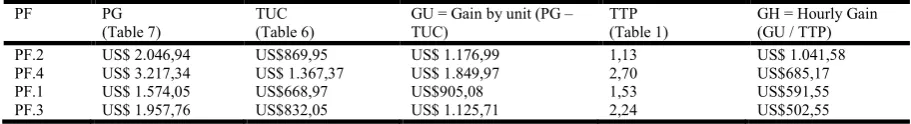
Recalling that this work was developed for small entrepreneurs without great knowledge in management, however, as their expertise in the subject will advance, it may insert other statistical treatments such as regression analysis, determinant, among others. In order to finalize the operation according to the method (Figure 1), the calculations required by phase 2.3 and represented in Table 6were performed, initially extracting the raw material and packing information in the purchase invoices, considering that the tax regime adopted by the company is “Simples Nacional” (in Brazil), which means that there is no recovery of tax credit. All the data inserted up to Table 6 can be easily inserted into a spreadsheet and processed in an integrated way, which means that when a cell is changed, the corresponding ones will be changed. Thus, the phases represented by Figure 1 and in this work converted into tables differ from the work of Morgado (2003) and Farias and Lembeck (2005), for simplifying the method in terms of form and content, partially meeting the premise (simplification of methods ) that guided this work. In order to confirm what was described in the first sentence of the introduction of this work, it was necessary to go beyond what is determined by the PEU method and for that it was necessary to calculate the Price Guidance (PG), which corresponds to the addition of variable selling expenses (VVE), which is nothing more than the amount of taxes levied on sales, freight, financial charges, commission, profit margin, among others. The composition of the VVE that make up Table 7 will not be presented to preserve confidential company information. Using the mark-up splitter method, the PG was determined for each PF based on the division of the TUC (Table 6) by the fraction of VVE subtracted from an integer.
Therefore, with a ranking per product, the one that offers the highest gain is the PF.4 with US$ 1,849.97, however, if the same reasoning is applied at the hour worked, the best result will be in PF.2 with US$ 1,041.58. According to Goldratt (1990), the difference between the gain per unit produced and the hour worked makes perfect sense when dealing with the constraints according to the steps shown in Table 9. In this
sense, the company can use the construct of Pacheco et al.
(2012), promoting the application of DBR according to the restrictions established, and new performance indicators can be used from the tabulation of data presented until Table 8, however, the logical application of methods as defended by
RHEE et al. (2010) and al. (2015), will depend on the
maturity of the company regarding the use of both methods recommended in this study. Adding the logic defended by Suri (2010) and Godinho Filho and Saes (2013) to the result presented in Table 8 and to the construct of this work, we have a vision focused on agility rather than cost, so the main performance objective will be the rhythm of production, regardless of constraints as defended by Goldratt (1990). Therefore, both converge to the same opinion, that is, what matters is not only to reduce costs, but to raise them to the condition of maximum efficiency and performance. Thus, the result of Table 8 should be analyzed by the ranking in Table 9.Based on what is shown on Table 9, it is clear that the company, regardless of restrictions in its production system, should emphasize product 2 (PF.2), followed by the product family PF.4, PF.1 and PF.3. This vision will allow the entrepreneur not only to have the precise notion of which product offers him the best margin per hour worked, but also
can determine to the other processes that reach a goal based on what the determined performance for that product. Finally, Table 9 allows a very wide range of decisions, from the planning of what to produce according to the best PG, as well as the joint balancing of production, either for reasons already discussed in the PEU method, or by constraints identified by the TOC. It is important to state that the combination of methods was demonstrated in this section, however, it will be up to the entrepreneur to be satisfied or to continue in the search for more specific answers, expanding the use through the aggregation of new techniques and knowledge.
DISCUSSION
[image:6.595.68.527.86.140.2]This work started from the premise that simplification is the best way for small business owners, often lacking in knowledge and technical support, to use methods that help in cost management. Therefore, the objective was to demonstrate the feasibility of using the Cost-Restriction-Analysis (CRA) method, which consists in calculating the costs of transformation, managing limiting factors of production and consequently forming sales prices. This was possible through a case study in a small fitness industry through the combined application of the PEU and TOC method as a way of calculating the costs of transformation and managing the limiting factors of production by defining the gains, inserting in this context principles of QRM. The respective methods were demonstrated in nine tables presented in the previous section, which, as a physical product of this work, can be converted into a spreadsheet in an integrated way. This, in
Table 6. Phases 2.3: Cost of products based on the PEU method
Period 1 PF.1 PF.2 PF.3 PF.4
Cost of Unit Transformation – CUT - US$ 368,51 395,47 251,66 674,10
Raw Material - US$ 235,06 401,50 512,37 595,44
Packing- US$ 65,40 72,98 68,02 97,83
∑ -Total Unit Cost - TUC- US$ 668,97 869,95 832,05 1.367,37
[image:6.595.72.528.186.229.2]Source: prepared by the authors based on the research data
Table 7. Use of mark-up splitter for PG definition
Period 1 PF.1 PF.2 PF.3 PF.4
1 - Total Unit Cost (TUC - Table 6) - US$ 668,97 869,95 832,05 1.367,37
2 - Mark-up Divider (1-VVE) 0,425 0,425 0,425 0,425
[image:6.595.69.525.271.334.2](1/2) Price Guidance (PG) - US$ 1.574,05 2.046,94 1.957,76 3.217,34 Source: prepared by the authors based on the research data
Table 8. Determination of gains using TOC
PF PG
(Table 7)
TUC (Table 6)
GU = Gain by unit (PG – TUC)
TTP (Table 1)
GH = Hourly Gain (GU / TTP)
PF.1 US$ 1.574,05 US$668,97 US$905,08 1,53 US$591,55
PF.2 US$ 2.046,94 US$869,95 US$ 1.176,99 1,13 US$ 1.041,58
PF.3 US$ 1.957,76 US$832,05 US$ 1.125,71 2,24 US$ 502,55
PF.4 US$ 3.217,34 US$ 1.367,37 US$ 1.849,97 2,70 US$ 685,17
[image:6.595.71.527.373.435.2]Source: prepared by the authors based on the research data
Table 9. Determination of earnings using TOC and QRM principles
PF PG
(Table 7)
TUC (Table 6)
GU = Gain by unit (PG – TUC)
TTP (Table 1)
GH = Hourly Gain (GU / TTP)
PF.2 US$ 2.046,94 US$869,95 US$ 1.176,99 1,13 US$ 1.041,58
PF.4 US$ 3.217,34 US$ 1.367,37 US$ 1.849,97 2,70 US$685,17
PF.1 US$ 1.574,05 US$668,97 US$905,08 1,53 US$591,55
PF.3 US$ 1.957,76 US$832,05 US$ 1.125,71 2,24 US$502,55
principle, will allow the analysis of results by indicators quickly, avoiding rework, however its greatest benefit may be the condition of becoming a dashboard, much used in large companies to control planning.
Following this logic, another additional contribution to the methods can be evidenced by the insertion of the statistical analysis, through the coefficient of variation, which in a simple and practical way will generate a much broader and safer view on the variations in the cost of transformation, among other possibilities of the analyzes contained in the presented tables. The counterpoint between the gain per product and the hourly gain is another information for those who were unaware of cost management techniques, providing a more precise ranking for the treatment of restrictions in the management process, allowing a balance of business objectives with the market demands. Thus, both planning and production control can be improved, and each new decision is tested for the identification of constraints arising from equipment failures, supplies, or even lack of funding. Therefore, it is possible to affirm that the premise used by these researchers is feasible, represented by the simplicity of data collection and treatment, making it possible to state also that the objective of this work was reached, since the applicability in a case study with data of a company in operation, allowed the visualization of the combination of methods, allowing the calculation of the costs of transformation and administration, the limiting factors of the production through definition of the gains, reaching a new level called here Cost-Restriction-Analysis (CRA).The main limitation identified in this work was the time to collect the necessary data and required in phase 1.3 according to Figure 1. It is advisable to follow the construct presented in this work, a lot of dedication in collecting data, in terms of time and filter avoiding to work with distorted or inaccurate data. As future contributions, it is suggested to broaden the research on the applicability of the PEU method to TOC, especially with regard to the limitations of production, correlating them with indicators and ways of solving them. An interesting way to achieve this goal is through the application of Cost-Restriction-Analysis (CRA) in a technical procedure defined as action research.
REFERENCES
Allora, V. 1996. UP’–Production Unit, a new method to
measure cost and industrial controls. In: 1st International
Conference on Industrial Engineering Applications and Practice. Houston, USA.
Barakchi, M., Torp, O., Belay, A. M. 2017. Cost Estimation Methods for Transport Infrastructure: A Systematic
Literature Review. Procedia Engineering, 196, pp.
270-277
Bozkurt, O. et al. 2014. The Importance of Cost Calculation
Method in the Accounting and Management of Turkish Operating Costs. A Research within the Scope of TAS-2. International Journal of Academic Research in Accounting, Finance and Management Sciences, 4 (2), pp. 38-46. Bruni, A. L., Famá, R. 2011. Gestão de custos e formação de
preços: com aplicações na calculadora HP 12C e Excel.Atlas,São Paulo, Brazil.
Deakin III, E. B. 1979. An analysis of differences between non-major oil firms using successful efforts and full cost
methods. Accounting Review, 34, pp. 722-734
Dos Santos, L. C. B. et al 2015. Profissionais da contabilidade
engajados no auxílio gerencial às micros e pequenas
empresas brasileiras. Revista Brasileira de Contabilidade, 210, pp. 56-69
Farias, V. M., Lembeck, M. 2005. Aplicação do método de custeio UEP em pequena empresa industrial. In: Anais do Congresso Brasileiro de Custos-ABC. Available on-line at: https://anaiscbc.emnuvens.com.br/anais/article/view/1881 Filippini, R. 1997. Operations management research: some
reflections on evolution, models and empirical studies in OM. International Journal of Operations & Production Management, 17 (7), pp. 655-670
Gitman, L. J. et al. 2015. Fundamentals of investing. Pearson
Higher Education, Houston, USA.
Godinho Filho, M; Saes, E. V. 2013. From time-based competition (TBC) to quick response manufacturing (QRM): the evolution of research aimed at lead time
reduction. The International Journal of Advanced
Manufacturing Technology. 64 (5-8), pp. 1177-1191
Goldratt, E. M. 1988. Computadorized Shop floor scheduling. Production Research, N.Y., USA.
Goldratt, E. M. 1990. The theory of constraints. North River Press INC., Croton-on-Hudson, NY.,USA.
Happ, H. H. 1994. Cost of wheeling methodologies. IEEE Transactions on Power systems, 9 (1), pp. 147-156
Horngren, C. T. et al 2009. Cost Accounting: a managerial
emphasis. Vol. 13.Pearson, São Paulo, Brazil.
Jeppsson, J., Sjöberg, J. 2017 Establishing a cost model when estimating product cost in early design phases. Available on-line at:http://www.diva-portal.org/smash/ record.jsf? pid=diva2:1136656
Johnson, W. B., Ramanan, R. 1988. Discretionary accounting 1970-76.Accounting Review, pp. 96-110
Morgado, J. F. 2003. Aplicação do método da UEP em uma pequena empresa de confecção de bonés: um estudo de caso. Thesis in Engineering of Production.Federal University of Santa Catarina, Florianópolis, Brazil.
Nascimento, E. Q., Mota, T. C. S., De Oliveira, D. L. 2015. Aplicação da TOC–Theory Of Constraints para tomada de decisão: Um Estudo de Caso em uma Industria Produtora de Bens de Capital com restrição de Capital. In: Anais do Congresso Brasileiro de Custos-ABC.
Pacheco, D. A. et al. 2012. Modelo de gerenciamento da
capacidade produtiva: integrando teoria das restrições e o índice de rendimento operacional global (IROG). Revista Produção Online, 12 (3), pp. 806-826
Pereira, N. A., Moura, M. F. 2016. Unidade de Esforço de Produção (UEP): Ferramenta Voltada para a Tomada de Decisão?RAGC, 4 (14), pp.100-112
Rhee, S. H., Cho, N. W., Bae, H. 2010. Increasing the efficiency of business processes using a theory of constraints. Information Systems Frontiers, 12 (4), pp. 443-455
Serajeldin, B. E. A., Jedo, A. A. A., Abdelraheem, A. A. E. 2017. Strategic Cost and Activating Competitive Advantage. International Journal of Trend in Scientific Research and Development, 1 (4), pp. 17-36
Smith, V. K. 2015 Should benefit–cost methods take account of high unemployment? Symposium introduction.Review of Environmental Economics and Policy, 9 (2), pp. 165-178
Sousa, R. 2005. Case research in operations management. EDEN Doctoral Seminar on Research Methodology in Operations Management. Bruxelas.
Suri, R. 1998. Quick Response Manufacturing: a
companywide approach to reducing lead times.
Suri, R. 2010. It’s about time: the competitive advantage for
quick response manufacturing. Productivity Press.
Portland, USA.
Sweeney, D. J., Williams, T. A., Anderson, D. R. 2011. Fundamentals of business statistics. Vol. 6. Cengage Learning. New York, USA.
Tanritanir, E. et al. 2004. Mobilyaimalatindafaaliyetmaliyet
leriyardimiylasimülasy ondesteklipersonelorganizasyonu. Gazi Üniversitesi Mühendislik-Mimarlık Fakültesi Dergisi, 19 (2), pp. 135-153
Wang, L. et al. 2009. Benefit evaluation of wind turbine
generators in wind farms using capacity-factor analysis and economic-cost methods. IEEE Transactions on Power Systems, 24 (2), pp. 692-704
Wernke, R., Junges, I. 2017. Nonfinancial indicators of the PEU Method applicable to the production management fridge. Custos e @gronegócio on line. 13 (1), pp. 35-52. Zimmerman, J. L. 2001 Conjectures regarding empirical
managerial accounting research. Journal of Accounting and
Economics, 32 (1), pp. 411-427