Comparing Bank Lending Channel in India and Pakistan

Munich Personal RePEc Archive

Comparing Bank Lending Channel in

India and Pakistan

Gupta, Abhay

University of British Columbia

November 2004

Online at

https://mpra.ub.uni-muenchen.de/9281/

Comparing Bank Lending Channel in India and Pakistan

– Abhay Gupta

University of British Columbia, Vancouver, Canada

Website:

http://grad.econ.ubc.ca/abhayg

Email:

abhayg@interchange.ubc.ca

Comparing Bank Lending Channel in India and Pakistan

This paper investigates the presence and significance of bank lending channel of the monetary policy transmission in India and Pakistan using the Structural Vector Auto Regression (SVAR) approach. The results of econometric analysis support the presence of a significant bank lending channel in these countries. Changes in the monetary policy instruments affect the credit variable (private sector claims) which in turn transmits the shocks to the real side of the economy, i.e. output and prices. The output returns back to initial level in long run, while the effect of monetary policy changes on prices are persistent.

The mechanism by which monetary policy is transmitted to the real economy

remains a central topic of debate in macroeconomics. Considerable research has recently

examined the role played by banks in the transmission of monetary policy aiming at

uncovering a credit channel and assessing the relative importance of the money and credit

channels.

1

Distinguishing the relative importance of the money and credit channels is

useful for various reasons. First, understanding which financial aggregates are impacted

by monetary policy would improve our understanding of the link between the financial

and the real sectors of the economy. Second, a better understanding of the transmission

mechanism would help monetary authorities and analysts to interpret movements in

financial aggregates. Finally, more information about the transmission mechanism might

lead to a better choice of intermediate targets.2 In particular, if the credit channel is an important part of the transmission mechanism, then the banks’ asset items should be the

focus of more attention.

This paper focuses on determining the presence and significance of the bank

lending channel for India and Pakistan.

Various econometric methodologies can be used to identify the presence and

significance of this channel.3 The traditional dynamic simultaneous model approach uses the system of equation to define a set of endogenous variables in terms of exogenous

variables and lags of endogenous variables. One of the major problems in this approach is

the difficulty of identifying truly exogenous variables that can be used as instruments.

variable has no influence on another variable. That is, there are hardly any compelling

identifying restrictions.

In response to these difficulties, Structural Vector Auto Regression (SVAR)

models treat all variables as endogenous. The sampling information in the data is

modeled with the help of VAR models, which model each variable as a function of all

other variables. Having modeled the reduced form of the model with the help of a VAR

system, the SVAR analysis proceeds to identify the model. To this end a ‘reaction

function in surprises’ is modeled, which expresses unexpected changes in the policy

instrument as a function of unexpected changes in the non-policy variable and of

monetary policy shocks. The objective is to identify the monetary policy shocks from this

relation, whichrepresent the discretionary component of policy.

Given these advantages, the paper also uses the SVAR methodology. Using the

data for the economies of India and Pakistan, a model is constructed consisting of

production, consumer prices, demand deposits, claims on private sectors, money (each in

log level), exchange rate, interest rate and spread. The model is analyzed using the

impulse responses and SVAR estimation (both short term and long term restriction results

are discussed).

The rest of paper is organized in following way. Some of the interesting facts and

figures about the unique banking structure of less developed countries are mentioned in

section I. It also provides brief history and current trends of banking sector in India and

Pakistan. The paper analyzes the different determinants of bank lending channel next.

Section II describes theoretical background behind bank lending/ credit channel in detail.

the econometric results. Then paper deals with the analysis of the effects of monetary

policy shocks on bank lending. Section 6 introduces the Vector Autoregressive

Regression (VAR) method in brief. Section 7 discusses the different econometric

approaches used to solve the identification problem. In section 8 a VAR model is setup

and then its estimation (using E-Views software) results are shown. Part IV of the paper

discusses and analyzes the results. The results of this paper for India and Pakistan are

compared with results from developed and other developing countries. The paper

concludes with summarizing the findings and mentioning the directions for future work.

I.

Descriptive

Statistics

Many of the recent research papers have established the importance of financial

sector development for economic growth.4 They have found that measures of the size of the banking sector and the size and liquidity of the stock market are highly correlated

with subsequent GDP per capita growth. Moreover, emerging evidence suggests that both

the level of banking sector development and stock market development exert a causal

impact on economic growth. Recent financial crises in South East Asia and Latin

America further underline the importance of a well-functioning financial sector for the

whole economy. Some of the important highlights of the banking sector in “Less

Developed Countries” (as defined by World Bank) are noted below.

A) Stylized facts on Banking Sector in LDCs

Unlike the developed countries, the financial sector in developing countries (or

LDCs) is still not mature enough. This contrast is evident from various measures like the

size, activity and efficiency of financial intermediaries and markets. For example

commercial banking firms was 7419. Compared to this number of commercial banks in

India is 293 (source: Reserve Bank of India, June 2003) and the total number of

scheduled banks in Pakistan is 46, including 22 foreign banks (based on Banking

Statistics of Pakistan, 2002 & 2003, published by State Bank of Pakistan).

Based on the data from the World Bank and other sources, some stylized facts on

banking sectors (in Less Developed Countries) can be noticed easily.

1. The first major point that differentiates developing countries from developed

countries, such as United States, is the lack of legal enforcement of financial markets’

rules and regulations. In LDCs collateral is scarce and contract enforcement is weak.

There is less collateralizable wealth, which results in borrower being charged higher

interest rate or rationed out of the market all together. Similarly the information is

scarce. Hence the contracts are much harder to enforce and borrowers can wilfully

refuse to pay back a loan without legally enforceable recourse. Moreover, in most

LDCs, it is difficult to seize collateral, resell it and/ or to use legal action to collect

bad debt.

2. The other observation is about interest rates. Compared to developed countries,

developing countries have a lot of variations in interest rates. For example the real

interest rates on deposits are either very high (Brazil 47%) or very low (Zimbabwe

19%). The average real interest rate on deposits for less developed countries is around

10.9%, while it is just 6.3% for developed countries. But more striking is the variation

3. Another noticeable trend in LDCs is considerably high spreads and high interest rates

being charged on the loans. Some of the probable reasons for spreads being higher are

lack of enforceable and marketable collateral, high loan default probabilities and high

bank operation costs. The average spread for developed countries is around 4.4%

while it is 10.4% for LDCs. Similarly the variance for developed countries is just 4.6

compared to 65 for less developed countries.

4. In most LDCs, banks dominate the financial system; equity (stock) markets and

corporate bond markets remain very shallow, concentrated and illiquid. Stock market

value to GDP ratio in 2003 was 2.88 for US and 1.3 for UK, while for India and

Pakistan this ratio was 0.5 and 0.2 respectively.

5. The ratio of private sector loans to GDP is very low (around 10%) for LDCs as

compared to developed countries, where it is almost 60%. This along with the fact

that equity and debt markets are shallow in LDCs leads to the trend that firms in

LDCs are more likely to depend on internal finance.

6. As a consequence of all these factors, it is not possible for small private banks to

operate profitably in less developed countries. Hence central banks and government

banks are very powerful. For example, in 2003 the assets of three largest banks as a

share of assets of all commercial banks for India and Pakistan is quite high (0.48 and

0.57) compared to US and UK (0.28 and 0.27). This means that there are few large

banks dominating the banking sector rather than a large number of small and medium

sized banks in these countries.

As documented by these stylized facts, there are institutional differences between

two groups. Therefore, the paper attempts to investigate the bank lending channel in

atypical countries not examined in previous literature.

India and Pakistan are chosen as the representatives of these LDCs. These two

countries add few interesting directions to the study. Both the countries got independence

at the same time and had similar social and economic condition. But, India followed a

socialist approach to the economic development in the beginning opening the economy in

1990s while Pakistan has had an open market policy from start. Thus, the results for India

and Pakistan could be similar or contrasting or both. These countries offer the potential to

provide some insights into the relative merits of different policies.

B) Institutional background of the banking sector in Pakistan

Pakistan in the 1950s and 1960s had a liberalized banking structure open to both

foreign and domestic banks. However, this changed in the early 1970s when the

government decided to nationalize all private domestic banks in the country. The

nationalization was interesting in the sense that only the domestic banks were

nationalized. The foreign banks were left to operate as before, although limits were

placed on the size of their operation. As a result of this institutional history, all foreign

banks operating in Pakistan were set up as new banks, i.e. none of them were buyouts of

existing private domestic banks. By 1990 government banks dominated the banking

sector as they held 92.2% of total assets, while the rest belonged to foreign banks.

However, weaknesses and inefficiencies in the financial structure that emerged

after nationalization, finally forced the government to initiate a broad based program of

reforms in the financial sector in the beginning of 1991. These reforms included: (i)

and foreign banks, (iii) setting up of a centralized credit information bureau (CIB) to

track loan-level default and other information, (iv) issuance of new prudential regulations

to bring supervision guidelines in-line with international banking practices (Basel

accord), and (v) granting autonomy to the State Bank of Pakistan that regulates all banks.

As a result of these reforms, the country saw a spur of growth in the private (particularly

domestic) banking sector.

During the fiscal year 20036, even a strong 28.9 percent growth in net government borrowings from scheduled bank, and a stunning 284.9 percent rise in private sector

credit, could not contain downward trend in interest rates for the second successive year

– the weighted average auction yield for the benchmark 6- month T-bills fell 463 basis

points during the year, taking the cumulative decline for the two years to a massive 1090

basis points. Fiscal year 2003 was as an exceptionally good year for the banking sector,

as the important banking indicators witnessed further improvement over fiscal year 2002.

Deposits of the banking sector grew by 19.5 percent (or Rs 275.1 billion) over the already

strong double-digit increases in the preceding two years. This impressive deposit growth

was largely driven by the unprecedented increase in workers’ remittances, which reached

US$ 4.2 billion during FY03 – the highest one-year accumulation in the history of

Pakistan.

C) Evolution of the Indian Banking Sector

Independent India inherited a weak financial system. Commercial banks

mobilized household savings through demand and term deposits, and disbursed credit

primarily to large corporations. Indeed, between the years 1951 and 1968, the proportion

percent. This increase was at the expense of some crucial segment of the economy like

agriculture and the small-scale industrial sector. This skewed pattern of credit disbursal,

and perhaps the spate of bank failures during the sixties, forced the government to resort

to nationalization of banks in 1969.

However, despite the successes of bank nationalization in India, the banking

sector remained mired in problems, and was incompatible with the emphasis on a market

economy, which was gradually emerging as the dominant economic paradigm worldwide.

With economic reform emerging as the primary agenda of the central government in

1990, the banking-financial sector in India witnessed a significant degree of liberalization

since the early nineties. Between 1992 and 1997, interest rates were liberalized, and

banks were allowed to fix lending rates subject to a cap of 400 basis points over the

prime lending rate (PLR).

Monetary conditions closely tracked the evolution of real activity during

2002-037. The growth of food bank credit, inclusive of banks’ investments in non-Statutory Liquidity Ratio (non-SLR) instruments, was in consonance with the recovery of

industrial output. Credit expansion was facilitated by conditions of ample liquidity in

financial markets, engendered by massive capital inflows. Interest rates declined across

the spectrum in response to the easy liquidity conditions. On the other hand, currency and

deposit growth slowed down moderately reflecting the adverse impact of the drought on

rural incomes and the lowering of deposit rates by banks. Broad money growth reflected

these diverse impulses from real activity. Financial markets were flush with liquidity over

overhang. There was a general easing of market conditions in terms of turnover and rates,

the latter enabled by the accommodative monetary policy stance.

These observations, facts, figures and numbers present a very interesting picture

of economies of less developed countries. Existence of bank lending channel as an

independent monetary policy transmission mechanism in developed countries has been

shown by various researches. However this kind of literature is scarce for less developed

countries. This paper applies the established theories and econometric methodologies of

determining the presence and significance of bank lending channel for India and

Pakistan.

II: Determinants of Bank Lending Channel

Bank lending has been a major area of research in recent years due to its

importance and the issues surrounding it. For example, following changes in monetary

policy strong correlation between bank loans and unemployment, GNP, and other key

macroeconomic indicators is observed by Bernanke and Blinder (1992). However, such

correlations could arise even if the “bank lending channel” is not operative. Since

contraction of bank loans in the wake of tight money cannot be unambiguous evidence

for the lending view. This is primarily due to high correlation between monetary and

credit aggregates. When bank loans contract, deposits are also likely to contract.

Therefore, one can argue that a monetary tightening depresses aggregate demand through

the conventional money channel resulting in a decrease of demand for bank loans (i.e. the

money view). In other words, it is necessary to identify the shifts of the supply and

demand schedules in the bank loan market. Thus, the contraction of bank loans is

equivalence is called the ‘supply-versus-demand puzzle’. The supply-versus-demand

puzzle has made it common to test the lending view, particularly in the US literature, by

examining the responses of banks to monetary policy with micro-data on banks’ balance

sheets (e.g. Kashyap and Stein, 2000).

Hence unlike the traditional theory that emphasizes households’ preferences

between money and other less liquid assets, the new theory of monetary policy asserts

that the role of the banking sector is central to the transmission of monetary policy. The

bank lending channel can be summarized as the impact of monetary policy on the amount

and conditions of credit as supplied by the banking sector. Monetary policy actions get

transmitted to the real economy through these changes in the loan supply behavior of

banks.

A. Data Set and Preparation

To test the bank lending channel for India and Pakistan the paper uses the

macroeconomic data since micro-level data is not available. The Statistics Department of

the International Monetary Fund publishes the International Financial Statistics (IFS)

database8. The data used here is taken from the Country Tables of the International Financial Statistics for India and Pakistan. The data for interest rate, exchange rate, CPI,

bank loans, industrial production etc is taken on Quarterly basis. These series run from

Q1:1957 to Q1:2004, but some data is available only for few years in between. Hence the

effective estimation period varies.

For India interest rates available are Bank Rate, Money Market Rate and Lending Rate,

while for Pakistan Discount Rate, Money Market Rate, Treasury Bill Rate and

Industrial Production is used for India and Manufacturing Production is used Pakistan.

Money is used as the monetary aggregate and consumer prices are used as a measure of

general price level in the economy. Exchange rate against US dollar is also used to take

care of the external effects on the economy.

The data is analyzed and plotted to see if there are any obvious trends between

these variables. In both the countries the interest rates have fluctuated a lot and there

seem to be no clear directions of movement to determine the intended monetary policy

measures. But a general trend can be seen, for instance it starts slowly going up from

1960s to 1980s, and then a sudden jump in early 1990s with abrupt fall in late 1990s.

Similarly the consumer prices have constantly moved up with slope increasing

significantly after 1980s (as can be seen in figure 2).

Consumer Prices India 0.0 20.0 40.0 60.0 80.0 100.0 120.0 140.0 Q 1 1 957 Q 3 1 960 Q 1 1 964 Q 3 1 967 Q 1 1 971 Q 3 1 974 Q 1 1 978 Q 3 1 981 Q 1 1 985 Q 3 1 988 Q 1 1 992 Q 3 1 995 Q 1 1 999 Q 3 2 002 Consumer Prices PAKISTAN 0.0 20.0 40.0 60.0 80.0 100.0 120.0 Q 1 1 957 Q 3 1 960 Q 1 1 964 Q 3 1 967 Q 1 1 971 Q 3 1 974 Q 1 1 978 Q 3 1 981 Q 1 1 985 Q 3 1 988 Q 1 1 992 Q 3 1 995 Q 1 1 999 Q 3 2 002

Figure 2: Consumer Prices Movements

As discussed earlier, to test the bank lending channel view one needs to focus on

finding answers of the following questions.

1. Do banks change their supply of loans when monetary policy changes?

2. Does spending respond to changes in bank loan supply?

On analyzing the sample data for these questions, definite trends in different

macroeconomic variables can be spotted. For example in both countries money, demand

deposit and private sector claims move along together (figure 3). Similarly for Pakistan,

private sector claims and manufacturing production seem to be correlated. This

Figure 1: Money, Private Sector Claims and Demand Deposit

Figure 2: Private Sector Claims Vs. Output (Industrial / Manufacturing Production)

Notice that in figure 3, there is a small-period sudden drop in log deposit variables

during 1970 and again in 1980 for India. Interestingly, in 1970 the ruling regime changed

from Congress to Janata Party. The new government was expected to change all the

instability. This sudden drop may be due to that volatility. Similarly, in 1980 Congress

formed the government with a majority.

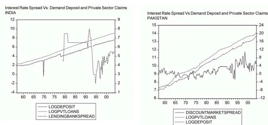
Similarly, a positive movement in the spread simply reflects that the monetary

tightening is inducing a fall in long-term rates, since there are expectations of a drop in

the short-term interest rate in the near future. On plotting different spreads, the effect of

interest rate movements on demand deposit and private sector claims does not seem to be

obvious.

Figure 3: Interest Rate Spread Vs. Deposits and Loans

These observations indicate the existence of few relationships between these

variables. The money and private sector loans are moving together for almost all of the

period. Similarly private sector loans and production are also moving together. This

suggests that over time changes in money are always accompanied by changes in private

sector loans and production, implying that these three variables are very closely related.

money are causing private sector loans to change which in turn is affecting the

production. But this simple analysis is not sufficient. Is it actually the changes in money

which cause private sector loans to change or both these are affected by some other

factors? There is a need to identify these relationships, to check if the relationships are in

agreement with the bank lending view and to see whether or not those are significant.

B. Preliminary Investigation

Proceeding further to investigate the bank lending channel in India and Pakistan, the

time series data mentioned in previous section is regressed to identify the presence and

significance of any relationships indicating the bank lending.

One of the issues involved in identifying the probable determinants of bank lending

channel is the “Problem of identification”, that is, without an exogenous shock to either

credit demand or credit supply, the system of two equations (one for credit supply and

another for credit demand) can not be estimated. For this to be properly resolved there

must be at least one variable present only in one of the supply or demand function

(Barajas & Steiner, 2002). The demand equation is identified if there is a variable present

in the supply equation that is not present in the demand equation. Similarly, the supply

equation is identified if there is a variable present in the demand equation that is not

present in the supply equation. Hence the major question becomes what macroeconomic

indicators can be taken as a measure of credit supply.

Due to non-availability of micro-level data, the loan demand and loan supply can not

be identified separately. The “claims on private sector” (monetary survey data of IFS

loans in these countries. It indicates the equilibrium value between loan demand and loan

supply. This is the “credit variable” used in this paper, representing the bank lending.

Another major assumption is that the paper treats money and interest rate both as

the monetary policy instruments in India and Pakistan. The reason is that the

governments of these countries have extensively used printing of new currency as a way

to finance the budget deficits. Unlike developed countries, the budget and the proposed

deficit have major impact on the economic decision making of agents in these countries

(especially for the case of India).

As mentioned in previous sections the flow of causality between the variables as

suggested by theory should be two folds. The changes in monetary policy should cause

changes in loan supply. This in turn should have significant effect on real economic

activity. Hence the major relationships for bank lending channel to be operative are:

1. Monetary Policy Instruments Æ Bank Credit

2. Bank Credit Æ Macroeconomic Activity

Two OLS regressions are run to identify the first relationship. The credit variable

(log private sector claims) is the dependent variable and each of the monetary policy

instruments (money, bank rate/ discount rate) is used as the explanatory variable. The

results are shown in table 1 below. Please note that private loans and money are in log

form. A time trend is also added in the second regression.

The second part of the channel is the affect of changes on this credit variable

(private loans) on real macroeconomic activities (industrial/ manufacturing

production).The results for simple OLS for this hypothesized relationship are shown in

India Pakistan

Dependant

Variable

Explanatory

Variable

Coefficient Explanatory

Variable

Coefficient

1. Pvt. Loans Money 1.246181

( 0.010057 )

R2 = 0.988095

Money 1.158518

( 0.012354)

R2 = 0.979177

2. Pvt. Loans Bank Rate 0.419237

(0.095012)

R2= 0.438146

Discount Rate 1.081293

(0.037859)

R2= 0.719822

Table 1: OLS results for effect of monetary policy on credit variable

India Pakistan

Dependant

Variable

Explanatory

Variable

Coefficient Explanatory

Variable

Coefficient

1. Production Pvt. Loans 0.358788

( 0.003492 )

R2 = 0.983874

Pvt. Loans 0.446374

( 0.005961)

R2 = 0.973950

On analyzing the above results, we find that:

1. Coefficient of relationship between money and private sector claims is significant,

and has a very high explanatory power (based on R-squared statistics).

2. Similarly coefficient of interest rate on private sector claims (loans) is significant,

but its explanatory power is not as high as that of the relationship with money.

The R2 is much smaller for the case of India.

3. The coefficient of private sector loans on production is significant and explains

most of the variations in the production.

The first two findings show that the relationships between monetary policy variables

and credit variable exist in these countries. However, the relationships of credit variable

with money are more significant than relationship of credit variable with interest rates.

Also the relationship between bank rate and credit variable is not very strong in India.

The last finding indicates that private borrowings affect the output (production). So

the relationship between macroeconomic activity and credit variable also exists in these

countries.

The paper now looks at different possible explanatory variables for this credit

variable, to check if there are any alternative relationships present in these economies.

Some of the obvious choices for explanatory variables (based on theoretical foundations

discussed above and on previous works) are Lending Rate, Deposit Rate, Spread,

overhead costs, GDP, inflation, stock market index, liquid liabilities (as % of assets),

lending capacity, non-performing loans or bank assets as % of central bank assets etc. But

that kind of data, this paper only uses money market rate, lending rate/ government bond

yield and the spread. The log value of credit variable (private sector claims) is regressed

on each of the above mentioned variables separately for both the countries. The results

for each regression are shown in table 3. A time trend is added in each regression.

On examining these relationships of credit variable with alternative instruments,

the spread seem to have some explanatory power for the movements in private sector

claims. However, the coefficient of determination for this relationship is less than the R2 with money as explanatory variable (which was around 0.98 for both the countries).

Similarly, the regression coefficients for other interest rates are significant, but have

small explanatory power.

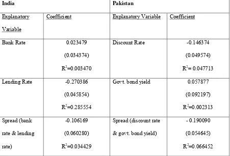
Till now the paper has used “private sector loans” as the indicator of bank lending

channel. Another indicator of bank lending may be “Investment Share of Gross Domestic

Product per Capita”. The argument is that movements in macroeconomic activities can

have a time trend associated with it, and this is especially true for the case of developing

countries. This would mean that changes in credit supply due to monetary policy shocks

may change the real macroeconomic activity via the investment share of GDP per capita.

Hence taking the percentage share of investment rather than the actual value of

investment may be a candidate for the credit variable. If there seem to be a significant

relationship between this variable and the monetary policy instruments, then this may

India Pakistan

Explanatory

Variable

Coefficient Explanatory

Variable

Coefficient

1. Lending rate - 0.509019

( 0.022782 )

R2 = 0.287015

Govt. bond yield 0.549185

( 0.031540)

R2 = 0.416377

2. Money market rate 0.352872

(0.030218)

R2= 0.436953

Money market rate 0.409181

(0.028160)

R2= 0.319804

3. Spread (bank rate &

lending rate)

-0.691344

(0.021061)

R2= 0.591561

Spread (discount

rate & govt. bond

yield)

0.516543

(0.046309)

R2= 0.308973

The data is taken from using the Penn World Tables9. Due to non-availability of the quarterly data, the yearly value is used for each of the four quarter. Separate regressions

are run to identify if this variable, has the relationships with any of the other possible

policy variables. The summary of least square regression results mentioning the

coefficients are shown in table 4.

The regression results indicate that bank interest rates or the spread does not have

any significant relationship with the investment share of per capita gross domestic

product. Hence this does not get affected by changes in monetary policy instruments and

thus not an indicator of bank lending channel in these countries.

To summarize, the preliminary investigation finds out that the credit variable

(private sector loans) has a very significant relationship with monetary policy instruments

for Pakistan. For India, the credit variable has a strong relationship with money but not

with the interest rate. Moreover, the credit variable has a very high explanatory power

(and significant relationship coefficient) with the macroeconomic activity (i.e.

production) for both countries. This indicates that bank lending channel is present in

these countries as a monetary policy transmission mechanism and it seems to be

significant. Interest rate does not seem to affect the credit supply effectively in case of

India. Any other alternative policy instrument - credit variable relationship does not seem

to be significantly present in these economies.

Given these encouraging indications, the paper proceeds to find out more detailed

information about the presence of bank lending in India and Pakistan by applying the

India Pakistan

Explanatory

Variable

Coefficient Explanatory Variable Coefficient

Bank Rate 0.023479

(0.034374)

R2=0.003470

Discount Rate -0.146374

(0.049574)

R2= 0.047713

Lending Rate -0.270386

(0.045854)

R2=0.285554

Govt. bond yield 0.057877

(0.092197)

R2=0.002313

Spread (bank

rate & lending

rate)

-0.106169

(0.060280)

R2=0.034429

Spread (discount rate

& govt. bond yield)

- 0.190090

(0.054645)

R2=0.066452

III: Effect of a MP Shock on Bank Lending

The VAR is a reduced-form time series model of the economy that is estimated by

ordinary least squares. Initial interest in VARs arose because of the inability of

economists to agree on the economy’s true structure.10 VAR methodologies11 for modeling the structure of an economy and issues involved in using those for the study of

monetary policy analysis have also been popular research topic.

A. Econometric Methodologies to the Analysis of Monetary Policy

The criticism of the reduced form model approach led to the development of

“Structural” VAR approach by Bernanke (1986), Blanchard and Watson (1986) and Sims

(1986). This technique allows the researchers to use economic theory to transform the

reduced-form VAR model into a system of structural equations. As discussed earlier a

VAR is a system where each variable is regressed on k of its own lags as well as on k lags

of the other variables (and a constant and a deterministic time trend, if necessary).

To discuss the SVAR approach to identification, the structural model of economy

is assumed to have the form –

ΓYt = B(L)Yt + et ……….(1)

where B (L) denotes polynomials in the lag operator L and Σe is the variance-covariance

matrix of the structural disturbances. The starting point of the SVAR analysis is the

reduced form of (1), which in matrix notation is given by –

Next, the moving average (MA) representation of the reduced form is computed, meaning

that the system is re-parameterized to express the endogenous variables in Ytas a function

of current and past reduced form innovations, ut. (ut = Γ-1 et ).

Yt = C(L) ut ………..(3)

with C(L) = ( I - Γ-1 B(L) )-1. A comparison of the MA representation with the conventional autoregressive (AR) representation shows that in the AR representation the

each variable is expressed as a function of past values of all the variables, whereas in the

MA representation each variable is expressed as a function of current and past

innovations in u.

Since no restrictions have yet been imposed on the model, it follows that the

impulse response functions given by C do not have any economic meaning. In other

words, even though they show the response of the economy to the reduced form

disturbance u, this is not particularly interesting because these disturbances are devoid of

economic content since they only represent a linear combination of the underlying

structural innovations e, given by ut = Γ-1et. Hence some restrictions need to be imposed

to get the real economic relationships and responses. These are known as identifying

restriction.12

The identifying restrictions used in the SVAR model can be categorized as

follows:

1. Orthogonality Restrictions

The identifying restriction that distinguishes the SVAR methodology from the

that the structural innovations are orthogonal, that is the covariance terms in Σe matrix are

zero. Since the reduced form disturbance is linked to the structural innovation by Γu=e,

the reduced form and the structural variance-covariance matrix are related to each other

by ΓΣuΓ-1=Σe. From this it follows that the orthogonality restriction imposed on Σe leads

to the non-linear restriction on Γ.

To explain the intuition behind the orthogonality restriction in SVAR models,

Bernanke (1986) writes that he thinks of the structural innovations “as ‘primitive’

exogenous forces, not directly observed by the econometrician, which buffet the system

and cause oscillations. Because these shocks are primitive, i.e., they do not have common

causes, it is natural to treat them as approximately uncorrelated.”

2. Normalization

SVAR models are based on the MA representation of the structural model, and

the empirical analysis seeks to estimate the impulse response functions. The impulse

response functions are usually computed to show the response of the model to a standard

deviation shock to the structural innovations. This makes it convenient to normalize the

SVAR model by setting the variances to one, because the standard deviation shocks, with

this normalization, correspond to unit innovations in e. From this follows that the

variance-covariance matrix of the structural innovations is Σe = I.

3. Restrictions on Relationship matrix

Finally exclusion restrictions are applied on matrix Γ for identifying the model

exactly. The reason for stressing on the analysis of Γ is that SVAR models aim to identify

the structural innovations e in order to trace out the dynamic responses of the model to

focuses on the relation Γut = et, and identifies the structural innovations by imposing

suitable restrictions on Γ. Hence in other words we can say that in SVAR models the

dynamic relationships in the economy are modeled as a relationship between shocks.

Any exclusion restriction on Γ automatically imposes a recursive order on the

system. This is called Choleski decomposition. Nevertheless, the Choleski decomposition

represents just one possible strategy for the identification of a SVAR model and should

only be employed when the recursive ordering implied by this identification scheme is

firmly supported by theoretical considerations. Alternatives include non-recursive

restrictions on the matrix Γ. Besides the restrictions on contemporaneous interactions it is

also possible to impose long-run restrictions on the effects of structural shocks. Finally, it

is also possible to combine contemporaneous and long-run restrictions.13

Contemporaneous versus Long-run Identification Schemes

A critical element in the estimation of the effects of policy shocks is the

identification of these policy shocks, i.e. the determination of exogenous shocks to

monetary policy. Two methods have been widely used in the VAR literature to identify

structural shocks to monetary policy. One general approach employs restrictions on the

contemporaneous relations among the variables of the vector autoregressive model, while

the second general approach imposes restrictions on the long-run relations among the

variables. Although economic and institutional arguments can be used to rationalize each

identification scheme, there is no consensus as to which approach to identifying shocks is

preferred, and the weaknesses of both approaches have been discussed in the research

papers. For example, the structural VAR method developed by Shapiro and Watson

form. Papers by Blanchard and Quah (1989) and Gali (1992) stress the fact that long run

restrictions are quite attractive for macroeconomic applications on real and nominal

variables. The reasoning behind this argument is that economic theory itself suggests that

nominal shocks have no long-run influence on real variables.

Interpretation of SVAR Analysis

It is tempting to use impulse response analysis to shed some light on the issue of

how long it takes until a change in the monetary policy stance reaches its full effect on

output, which is an important issue in applied business cycle analysis. But impulse

response analysis is unlikely to be helpful in this regard, because most monetary policy

actions represent a systematic response of the central bank to the state of the economy

and do not come as surprises. That is, most monetary policy actions are not monetary

policy shocks. It is therefore important for applied business cycle research to know what

the output effects of systematic monetary policy are, while the output effects of

unanticipated, discretionary monetary policy are only of secondary interest. But impulse

response analysis only says something about the latter aspects, and remains largely silent

on the output effects of systematic and hence anticipated monetary policy.

The shock analysis conducted in SVAR models is the closest approximation of a

controlled experiment available in empirical economics. Once the monetary policy shock

is identified, one can see the monetary transmission mechanism unfold by observing the

response of the non-policy variables to this monetary impulse. The issue of reverse

causality which usually plagues the analysis of dynamic relationships is not an issue in

SVAR models, because by tracing out the dynamics of the system to an unexpected

shock to the other variables in the model. This kind of structural inference is not possible

using the conventional reduced form analysis of the lead/lag structure, which is often

employed as an alternative tool to investigate the transmission mechanism.

B. Detailed Estimation

Before the specification of the VAR model for detailed estimation, it is important to

recall that three necessary conditions need to be satisfied conceptually for the bank

lending channel to be effectively operative.

1. Firms must not be able to easily substitute bank loans with commercial paper or

public equity (Kashyap, Wilcox & Stein, 1993).

2. Central bank must be able to affect the supply of loans (Gertler & Gilchrist,

1994).

3. There should be nominal price rigidity, so that monetary policy can have real

effects.

The third condition exists in most of the economies. Due to semi-regulated

environment of Indian and Pakistani economies (for example government decides the

price of many basic things like petrol, food-grains etc.), nominal price rigidity can be

assumed to be present. As mentioned in section about less developed countries’ banking

sector, the private bond and equity markets are still very immature in India and Pakistan.

Hence the first condition is also met easily, because it is not possible for firms to sought

loans from sources other than banks. The first condition, central bank’s ability to affect

the supply of loans, can not be determined due to lack of firm level data. The paper

however treats the changes in the private sector loans as the indication of changes in loan

affect this credit variable. Hence the third condition is also satisfied (somewhat weakly

for India).

The VAR model in this paper consists of the macroeconomic series and bank data

mentioned in previous part. The output is captured using the industrial or manufacturing

production as a proxy for the macroeconomic activity. The annual currency depreciation

is included using the exchange rate and movements in relative prices are captured by

consumer prices. These two variables are intended to control for demand side of the

economy. Similarly money and interest rate are used for money market and instrument of

monetary policy. To identify the changes in loan demand and loan supply, claims on

private sector and demand deposit are included in the system. The spread is also

introduced in the model to disentangle the supply and demand.

In a VAR, all contemporaneous correlation between two variables is attributed to the

variable higher in the ordering. The paper uses a the following ordering –

1. Log production. 2. Log CPI. 3. Log deposit. 4. Log Pvt. Loans.

5. Exchange rate. 6. Spread. 7. Interest rate. 8. Log money.

This kind of ordering is justified using the fact that since Bank Rate and Money are the

policy variables, shocks in these affect output and prices with a lag via the changes in

deposit, loans and exchange rate.

1. Unrestricted VAR Estimation

First, the unrestricted VAR model is estimated to further analyze the presence of

bank lending channel and its role in transmission of monetary policy shocks.

The lag length selection tests for India suggested using either 4 (the sequential

criteria) lags. For Pakistan the ideal lag length suggested by tests (LR, FPE, AIC) is 5 or

1 (SC). Since using four lag also takes care of seasonality in the quarterly data being used

here, the optimal number of lags is taken as 4.

The VAR models for both the countries are stable. Since all the AR roots have

modulus less than one and lie inside the unit circle.

To assess the importance of bank lending channel one needs to test for the marginal

predictive power of the “credit variable” by carrying out Granger causality tests14. This evidence alone is not sufficient. It has to be complemented with two simultaneous

conditions:

• The money and/ or interest rate (or term spread) is relevant for predicting the

credit variable, signifying the monetary policy affecting the bank lending.

• This credit variable should be relevant for explaining the macroeconomic activity

variable, implying that this channel has transmitted the monetary policy changes

to real economy.

1.1 Pair-wise Granger Causality15

The simplest way to get the answer for the question “does the bank lending channel

play any significant macroeconomic role as monetary policy transmission mechanism” is

to analyze whether private sector claims in our model adds any explanatory power to any

of the macroeconomic variables. The results for the pair-wise granger causality using the

diagnosis of VAR lag structure are shown below. The number indicates the p-value based

on the Wald statistics for the joint significance of each of the other lagged endogenous

variables in the equation. The null hypothesis for the pair production – private (shown in

1. INDIA:

Production

Exclude Prices Exchange

Rate

Pvt.

Loans

Deposits Money Spread Bank

Rate

All

Prob. 0.3730 0.0001 0.6466 0.1120 0.0001 0.5724 0.1020 0.0000

Prices

Exclude Production Exchange

Rate

Pvt.

Loans

Deposits Money Spread Bank

Rate

All

Prob. 0.0239 0.1717 0.8930 0.2551 0.2660 0.8783 0.8646 0.0000

2. PAKISTAN:

Production

Exclude Prices Exchange

Rate

Pvt.

Loans

Deposits Money Spread Bank

Rate

All

Prob. 0.1345 0.0072 0.0728 0.6298 0.3802 0.2942 0.2560 0.0000

Prices

Exclude Production Exchange

Rate

Pvt.

Loans

Deposits Money Spread Bank

Rate

All

Prob. 0.0002 0.1772 0.1828 0.0145 0.0571 0.2221 0.6829 0.0000

A high p-value does not reject the null hypothesis, while a low p-value (less than

10%) rejects the null hypothesis. The results seem to indicate that private loans granger

cause output in Pakistan. This re-iterates the earlier results about the existence of

relationship between private loans and production in Pakistan. While for India, the null

can not be rejected. Hence, it can not be said that private sector loans causes production.

But since Granger causality measures precedence and information content but does not

by itself indicate causality in the more common use of the term. The rejection of null

does not mean that there is no relationship between private loans and production. Hence,

the Granger causality result for India is ignored. The paper still treats previous part’s

results as established for both the countries.

Finally, the unrestricted VAR estimation is done using 4 lags of each endogenous

variable in the model. On examining the relevant relationship coefficients, the lagged

values of “monetary policy” variables (money and interest rates) are significant in

predicting the credit variable (private sector claims) for both the countries. The

coefficients of the interest rate are not as significant as those of the money. The credit

variable (and its lags) also seems very significant in explaining the macroeconomic

variables.

Thus, the unrestricted VAR also indicates that there is bank lending channel

present in these countries.

1.2 Impulse Responses

A shock to the policy variable not only directly affects that variable but is also

transmitted to all of the other endogenous variables of the economy through the dynamic

monetary policy shock to one of the innovations on current and future values of these

variables.

Responses of Macroeconomic variables (Output, Prices) to Cholesky One S.D.

Innovations in Policy variables (Money, Interest Rate) along with responses of

intermediate credit variables (loan demand and loan supply) are shown in figure 6 and

figure 7.

The cholesky impulse is used, which imposes an ordering of the variables in the

VAR and attributes all of the effect of any common component to the variable that comes

first in the VAR system. The graph shows the plus/minus two standard error bands about

the impulse responses.

One important thing to notice is that as a result of positive innovation in money

the mean response of private loans goes down (the usual predicted response is that loans

should go up). However, a zero response lies within the two standard deviation band.

As is clear from figure 6 and 7, these impulse responses show that for both India

and Pakistan shocks in interest rates and money affect output and prices. While the output

returns to initial level, the effects on prices are persistent. The shocks in interest rates and

money also affect the credit variable, it goes down and then goes up (further than initial

level). The final level of credit variable after the interest rate shock is above the initial

level for Pakistan (while for India it is somewhat below the starting value). Basically, the

figures show changes in money induce a change in private sector loans and the real

-.012 -.008 -.004 .000 .004 .008 .012 .016 .020

1 2 3 4 5 6 7 8 9 10

Response of LOG PRODUCTION to LO GMONEY

-.012 -.008 -.004 .000 .004 .008 .012 .016 .020

1 2 3 4 5 6 7 8 9 10

Response of LO GPRODUCTION to BANKRATE

-.008 -.004 .000 .004 .008 .012 .016

1 2 3 4 5 6 7 8 9 10

Response of LOGCPI to LOGMONEY

-.008 -.004 .000 .004 .008 .012 .016

1 2 3 4 5 6 7 8 9 10

Response of LO GCPI to BANKRATE

-.016 -.012 -.008 -.004 .000 .004 .008 .012

1 2 3 4 5 6 7 8 9 10

Response of LOGPVTLOANS to LOGMONEY

-.016 -.012 -.008 -.004 .000 .004 .008 .012

1 2 3 4 5 6 7 8 9 10

Response of LO GPVTLO ANS to BANKRATE

-.02 -.01 .00 .01 .02 .03

1 2 3 4 5 6 7 8 9 10

Response of LOGDEPOSIT to LOGMONEY

-.02 -.01 .00 .01 .02 .03

1 2 3 4 5 6 7 8 9 10

Response of LOG DEPOSIT to BANKRATE

Response to Cholesky One S.D. Innovations ± 2 S.E.

-.03 -.02 -.01 .00 .01 .02

1 2 3 4 5 6 7 8 9 10

Response of LOG PDN to LOGMONEY

-.03 -.02 -.01 .00 .01 .02

1 2 3 4 5 6 7 8 9 10

Response of LO GPDN to DISCOUNTRATE

-.01 .00 .01 .02 .03 .04

1 2 3 4 5 6 7 8 9 10

Response of LOG CPI to LOGMONEY

-.01 .00 .01 .02 .03 .04

1 2 3 4 5 6 7 8 9 10

Response of LO G CPI to DISCOUNTRATE

-.02 -.01 .00 .01 .02 .03 .04

1 2 3 4 5 6 7 8 9 10

Response of LO GDEPOSIT to LO GMONEY

-.02 -.01 .00 .01 .02 .03 .04

1 2 3 4 5 6 7 8 9 10

Response of LO GDEPO SIT to DISCOUNTRATE

-.02 -.01 .00 .01 .02 .03

1 2 3 4 5 6 7 8 9 10

Response of LOGPVTLOANS to LO GMONEY

-.02 -.01 .00 .01 .02 .03

1 2 3 4 5 6 7 8 9 10

Response of LO GPVTLO ANS to DISCOUNTRATE

Response to Cholesky One S.D. Innovations ± 2 S.E.

Hence the impulse responses indicate that the bank lending channel seem to be

operative and the shocks in money and interest rates are transmitted to the real side of

economy (output and prices) via the changes in private loans (credit variable). These

observations are in agreement with previous results, indicating the presence of bank

lending.

1.3 Variance Decomposition

While impulse response functions trace the effects of a shock to one endogenous

variable on to the other variables in the VAR, variance decomposition separates the

variation in an endogenous variable into the component shocks to the VAR. Thus, the

variance decomposition provides information about the relative importance of each

random innovation in affecting the variables in the VAR.

The variance decomposition of the VAR model shows that exchange rate and

money play more important role than interest rate or term spread in determining the

private sector claims. Similarly an innovation in private sector claims affects the

production somewhat significantly, but not the price levels. The results are alike for both

the countries and are in agreement with previous results.

2. Structured (Identified) VAR

The main purpose of structural VAR (SVAR) estimation is to obtain

non-recursive orthogonalization of the error terms for impulse response analysis. This

alternative to the recursive Cholesky orthogonalization requires the user to impose

enough restrictions to identify the orthogonal (structural) components of the error terms.

2.1 Short Term restrictions

1. output 2.cpi 3.deposit 4. loans

5.exchange-rate 6.spread 7.interest rate 8.money

This kind of identification scheme is used by other researchers as well (McMillin,

1999). The assumption that monetary policy affects output and prices only with a lag and

that it has a contemporaneous effect upon the exchange rate is uncontroversial. With

same kind of reasoning monetary policy will have more immediate effect on private

sector loans and demand deposit (since monetary policy affects these variables first,

which in turn transmit the monetary shocks to the real economy).

The SVAR is identified by specifying the standard short run restriction matrices.

That is for the relationship ut = Γ-1et, between reduced form and structural disturbances,

Γ-1

is restricted as the lower triangular matrix.

The impulse response results are shown in figures 8 and 9.

Notice that, the “credit variable” gets affected by shocks in either of the monetary

policy instruments, and gets back to its initial level. The same is true for the output levels.

But for both the countries, this identification scheme shows a permanent effect of

monetary policy on consumer prices for both the countries. So the results of this SVAR

analysis are similar as the earlier results.

2.2 Long Run restrictions

One advantage of the use of LR is that no restrictions are placed on the

contemporaneous relations among the variables. Thus, a restriction that monetary policy

shocks have no contemporaneous effects on output or prices is not imposed, as was done

-.004 .000 .004 .008 .012

1 2 3 4 5 6 7 8 9 10 LOGMONEY BANKRATE Response of LOGPRODUCTION to Cholesky

One S.D. Innovations

-.002 .000 .002 .004 .006 .008

1 2 3 4 5 6 7 8 9 10 LOGMONEY BANKRATE Response of LOGCPI to Cholesky

One S.D. Innovations

-.006 -.004 -.002 .000 .002 .004

1 2 3 4 5 6 7 8 9 10 LOGMONEY BANKRATE Response of LOGPVTLOANS to Cholesky

One S.D. Innovations

-.004 .000 .004 .008 .012 .016

1 2 3 4 5 6 7 8 9 10 LOGMONEY BANKRATE Response of LOGDEPOSIT to Cholesky

One S.D. Innovations

Figure 6: Impulse Response of SVAR with Short Run restrictions for INDIA

-.012 -.008 -.004 .000 .004 .008

1 2 3 4 5 6 7 8 9 10 LOGMONEY DISCOUNTRATE Response of LOGPDN to Cholesky

One S.D. Innovations

-.004 .000 .004 .008 .012 .016 .020

1 2 3 4 5 6 7 8 9 10 LOGMONEY DISCOUNTRATE Response of LOGCPI to Cholesky

One S.D. Innovations

-.004 .000 .004 .008 .012 .016 .020

1 2 3 4 5 6 7 8 9 10 LOGMONEY DISCOUNTRATE Response of LOGDEPOSIT to Cholesky

One S.D. Innovations

-.008 -.004 .000 .004 .008 .012

1 2 3 4 5 6 7 8 9 10 LOGMONEY DISCOUNTRATE Response of LOGPVTLOANS to Cholesky

One S.D. Innovations

The first restriction used to identify the monetary policy shock is that money or

interest rates shocks have no long-run effects on output. A second restriction is that

monetary policy shocks have no long-run effects on the interest rate. These are familiar

results from a sticky-wage/price aggregate demand-aggregate supply-type model with

IS-LM underlying aggregate demand. Interest rate and spread are not affected by any of the

other variables. It is also assumed that exchange rate or price level does not have any

influence on output in long run.

The model is estimated applying these long run restrictions. The results of

estimations (the matrix Γ-1) are as shown in tables 7 and 8. The coefficient in each cell

represents the contemporaneous relationships of error terms/ shocks of row variable with

the different column variables.

As can be seen from these tables, private sector loans have a positive relationship

with the shocks in money (and negative relations with shocks in interest rate and spread).

The changes in the private sector claims affect the output positively. The results show

that the relationships of policy instruments with credit variable and of credit variable with

macroeconomic activities exist in these economies.

Impulse responses for this identification are similar to the ones obtained from

contemporaneous restrictions earlier.

Hence the detailed estimation, again affirms the preliminary investigation results

of bank lending channel being present in these countries as a mechanism of monetary

policy transmission. It reveals that shocks in the policy instruments (interest rates and

money) transmit to the macroeconomic activities (production and prices) of these

Estimated Relationship matrix: INDIA

Output Prices Exchange

Rate

Pvt. Sector

Loans

Deposits Money Spread Interest Rate

Output -0.409397 (0.019335) -0.456411 (0.005022) -0.020028 (0.003028) -0.495360 (0.060161) 0.625472 (0.002394) -0.441435 (0.022934) 0.003789 (0.086403) -0.000865 (0.059351) Prices -0.001042 (0.004691) -0.011334 (0.059351) -0.007838 (0.065948) -0.234446 (0.098731) 0.011189 (0.019856) -0.003741 (0.008329) -0.003790 (0.050527) -0.000523 (0.003305)

Exchange Rate 4.985983

(0.085794) 5.557096 (0.030483) 0.179344 (0.004653) 6.029751 (0.069745) -7.552790 (0.024772) 4.484849 (0.003236) 0.159798 (0.046723) -0.408838 (0.054246) Pvt. Sector Loans 0.036271 (0.057635) 0.043570 (0.047625) 0.007153 (0.006423) 0.041001 (0.050385) -0.041820 (0.067574) 0.758432 (0.043593) 0.018747 (0.003785) -0.207678 (0.002368) Deposits -0.533826 (0.064862) -0.600091 (0.007534) -0.012034 (0.003541) -0.665065 (0.004924) 0.876585 (0.070456) -0.596376 (0.003588) 0.021716 (0.075623) 0.036462 (0.004763) Money -0.206352 (0.076357) -0.241505 (0.004562) -0.001950 (0.067635) -0.277660 (0.009471) 0.342680 (0.034565) -0.251694 (0.006523) 0.005550 (0.007024) 0.011635 (0.069913)

Spread 3.206759

(0.068624) 3.458569 (0.013028) 0.109651 (0.063052) 3.718781 (0.053274) -5.164326 (0.049748) 3.130781 (0.079725) 0.243803 (0.019539) 0.062175 (0.004783)

Interest Rate -1.197172

(0.007551) -1.054037 (0.045642) -0.190304 (0.029475) -1.404653 (0.054656) 1.929425 (0.009431) -1.138668 (0.089134) -0.142652 (0.064052) -0.016091 (0.005406)

Estimated Relationship matrix: PAKISTAN

Output Prices Exchange

Rate

Pvt. Sector

Loans

Deposits Money Spread Interest

Rate

Output 0.000276

(0.006405) 0.003437 (0.049164) 0.004330 (0.050236) 0.277891 (0.002057) 0.026869 (0.004531) -0.042037 (0.096291) -0.039933 (0.005491) 0.034302 (0.015374)

Prices 0.014752

(0.020436) 0.009095 (0.003465) 0.002062 (0.005759) 0.310291 (0.054124) -0.003242 (0.067651) 0.019144 (0.009128) 0.002948 (0.007431) -0.012067 (0.065625)

Exchange Rate 0.158459

(0.068545) 0.335979 (0.043769) -0.179822 (0.003215) -2.669775 (0.013400) -0.998229 (0.006052) 1.243500 (0.054766) 0.732730 (0.004334) -0.153593 (0.072064) Pvt. Sector Loans -0.006401 (0.001605) -0.001878 (0.004306) -0.006972 (0.001204) -0.022109 (0.005465) -0.027566 (0.034306) 0.540360 (0.095230) -0.012212 (0.003651) -0.402790 (0.002854) Deposits -0.037021 (0.033954) -0.036409 (0.007504) 0.006903 (0.009020) 0.077049 (0.054763) 0.041400 (0.006932) -0.067809 (0.082062) -0.051723 (0.005004) -0.004009 (0.045043) Money -0.017751 (0.056690) -0.001982 (0.004946) 0.002578 (0.003651) 0.006497 (0.004595) 0.003402 (0.003910) 0.013366 (0.045737) -0.011522 (0.002307) 0.001276 (0.006524) Spread -0.072563 (0.043065) 0.548751 (0.000551) -0.291594 (0.019340) -0.217812 (0.006523) 0.042878 (0.008430) -0.120213 (0.061302) -0.088930 (0.005641) -0.116240 (0.020548)

Interest Rate 0.014761

(0.073062) 0.447960 (0.058302) -0.492315 (0.006103) -0.369468 (0.008209) 0.104915 (0.035052) -0.025117 (0.009305) 0.005054 (0.041121) -0.084015 (0.072503)

D. Explanations and Analysis of Results

The results of econometric analysis in previous two parts should be analyzed

keeping basic economical structure and the macroeconomic policies of these two

countries in mind. While there has been evidence of association between movements in

interest rate (or yield spread, to be more precise) and real economic activity in most of

the developed countries, these kinds of results are virtually absent in the case of

developing economies. In part, this is because in developing economies with

administered interest rates yield curve has not been market determined. Moreover, both

the countries started as agricultural economies with not very developed banking system

and have struggled even with the stability of political regimes (especially in the case of

Pakistan). Hence one can reason why the results for interest rate as monetary policy

instrument are not as apparent as in case of developed countries. Even the presence of

informal credit market, which is operable mostly in rural economies (forming a large

percent of total till late 1980s), can be blamed for usual monetary policy shocks (interest

rates) not affecting the loans that much.

As mentioned earlier, the other important point to consider is that unlike

developed countries, India and Pakistan have sought to printing of currency as a measure

to finance the government deficit. Hence usual open-market operations loose some of the

significance in impacting the real macroeconomic activity via credit channel.

Now the results are compared with previous such works on the bank lending

1. Comparison with Developed Countries

Perhaps the simplest aggregate empirical implication of the bank-centric view of

monetary transmission was suggested by Bernanke and Blinder (1992). They showed that

for US, following changes in monetary policy, there is a strong correlation between bank

loan and key macroeconomic indicators like unemployment, GNP etc. The simple OLS

results in part-II show that this kind of aggregate level relationship exists in India and

Pakistan.

The presence and significance of bank lending channel as monetary policy

transmission mechanism in developed countries like US, Canada or other European

countries has been established by many research papers in past. These papers used

different indicators or proxies for bank lending. For example, ‘ratio of bank vs. non-bank

debt’ is observed to decline positive innovation in the federal fund rates16.

In this paper due to availability of only aggregate level financial data, the credit

variable used is “private sector claims”. The results show that there exists a significant

relationship between this credit variable and macroeconomic activity (production). The

levels of significance of bank lending channel shown in studies for developed countries

should not be compared with results in this paper, because the credit variables used are

different. However, one fact to note is that the effect of interest rate shocks on the credit

variable is not as significant as the effect of a shock in money supply.

Another most commonly used variable, term spread has been shown to explain

the presence of credit channel for the developed countries. Again since interest rate is not

a very effectively used instrument in India and Pakistan, the spread does not seem to have

a good indicator of bank lending channel for India and Pakistan (unlike the results from

developed countries, where the spread is very promising credit channel variable).

There are similarities in results of impulse response and variance decomposition

analysis for these two countries and developed countries like US, Canada. The effect of

monetary policy shock on output gradually dies, and output reaches the initial

equilibrium level, while changes in prices are persistent.

2. Comparison with other Developing countries

Agung (1998)17 finds significant different responses across the bank-size classes to a change in monetary policy for Indonesia. In particular, a monetary contraction does

not significantly influence lending by state banks, but it leads to a decline in lending by

smaller banks. A lot of papers have focused on discussing the bank lending channel in

European countries like Spain, Poland, and Sweden18 etc. Again many of these studies have been done on the micro level bank panel data, which unfortunately is not available

for the case of this paper. But on aggregate level the results for India and Pakistan also

suggest that a monetary policy shock induced by changes in money supply leads to

changes in private sector loans, as is the case with many of the developing countries.

Whether there is a distributional aspect of this relationship can not be inferred from this

study due to data constraints.

For Sweden households and firms are found to be constrained to bank lending,

which imply that any policy induced shifts in the supply of bank loans should also cause

real spending effects19. Similarly, it is observed that banks are significantly deposit constrained and that they have only limited access to external forms of finance, which

growth. Similar studies have been done for Latin American countries like Chile, Brazil

etc.20 For Chile Alfaro, Franken, García and Jara (2003) use the panel data of banks to identify the presence of bank lending channel. They introduce a new variable (low/ high

quality ratio) to capture the asymmetric nature of different financial agents. But most of

the studies have either focused just on identifying the determinant of bank lending using

bank panel data or stressed only on analyzing the effects of monetary policy shocks on

bank lending using macroeconomic series.

This paper is unique in the sense that it attempts to address the both issues and

create the complete picture of the economy vis-à-vis bank lending channel as

transmission mechanism of monetary policy. Private sector loan is used as the credit

variable and seem to have marginal predictive power on other macroeconomic variables.

Hence the bank lending channel is present in India and Pakistan. The monetary policy

shocks (specially the ones in money supply) are transmitted to real economic activities

via this channel.

3. Contrasts between India and Pakistan

The results for India and Pakistan are similar in most of the aspects. Both the

countries have bank lending channel present in their economies and it is a significant

transmission mechanism for monetary policy shocks. For both the countries money

supply appears to be the more effective in affecting the macroeconomic activities (via

credit variable) rather than interest rate. But the discount rate in Pakistan appears to be

much significant instrument that the bank rate in India. This may be attributed to the fact

that Pakistan has a more market oriented and liberal policies compared to India which