Financial development and economic growth: The case of eight Asian countries

(1)

Munich Personal RePEc Archive

Financial development and economic

growth: The case of eight Asian countries

Sinha, Dipendra and Macri, Joseph

Ritsumeikan Asia Pacific University, Japan and Macquarie

University, Australia, Macquarie University, Australia

2001

Online at

https://mpra.ub.uni-muenchen.de/18297/

(2)

FINANCIAL DEVELOPMENT AND ECONOMIC GROWTH: THE CASE OF EIGHT ASIAN COUNTRIES

Dipendra Sinha, Macquarie University and Yale University

Department of Economics Macquarie University

Sydney, NSW 2109 AUSTRALIA

E-mail: dipendra.sinha@efs.mq.edu.au

and

Joseph Macri, Macquarie University

Department of Economics Macquarie University

Sydney, NSW 2109 AUSTRALIA

E-mail: joseph.macri@efs.mq.edu.au

ABSTRACT

This paper looks at the relationship between financial development and economic growth using time series data for eight Asian countries. First, we estimate augmented production functions where a financial development variable is added. Second, we conduct

multivariate causality tests between the growth rate of income and the growth rates of the financial development variables. The regression results show a positive and significant relationship between the income variables and financial variables for India, Malaysia, Pakistan and Sri Lanka. The multivariate causality tests show a two-way causality relationship between the income and the financial variables for India and Malaysia, one-way causality from financial variables to income variables for Japan and Thailand and reverse causality for Korea, Pakistan and Philippines. Thus, our empirical results do not unambiguously support the general view of a clear and positive relationship between financial development and economic growth.

JEL Classification: C32, E51, O10

(3)

1. Introduction

A large number of studies have analysed the relationship between financial sector

development and economic growth. These studies have included both time series and

cross section data. The main objective of this study is to examine the relationship

between financial sector development and economic growth for the following Asian

countries: India, Japan, Korea, Malaysia, Pakistan, Philippines, Sri Lanka and Thailand.

A number of features distinguish this study from all other existing time series studies.

First, we test for the presence of unit root(s) before proceeding with the estimation.

Second, we employ a much longer time series data set. Third, we perform multivariate

causality tests, which no other previous studies have undertaken. If the evidence suggests

that causality exists from financial sector development to economic growth then this has

direct policy implications. Generally, the literature thus far has implied that a more

efficient financial system will provide “better” financial services, which will enable an

economy to increase its real GDP growth rate. Therefore, establishing appropriate

financial sector policies are of paramount importance to policymakers. Such policies, it is

argued, will ameliorate market failures − by providing services that facilitate transactions,

mobilize capital, exert corporate governance − which are important for economic growth.

Our sample includes seven developing countries and a developed country (Japan). The

inclusion of Japan is to determine whether there is a difference in the relationship

between financial sector development and economic growth in Japan versus other

(4)

2. Theoretical and Empirical Literature Review

A large and diverse body of theoretical and empirical literature has investigated the

importance of the financial sector for economic growth. This work can be traced as far

back as Bagehot (1873), Schumpeter (1912) and Hicks (1969). More recent work

includes Levine (1998), King and Levine (1993a, 1993b), Rousseau and Wachtel (1998),

Rajan and Zingales (1998), and Okedokun (1998). Bagehot (1873) and Hicks (1969), for

example, argued that the financial system was an important catalyst in the

industrialization of England by facilitating the movement of large amounts of funds for

“immense” works. Bagehot (1873, pp. 3-4) observed:

“We have entirely lost the idea that any undertaking likely to pay, and seen to be likely, can perish for want of money; yet no idea was more familiar to our ancestors, or is more common in most countries. A citizen of London in Queen Elizabeth’s time … would have thought that it was no use inventing railways (if he could have understood what a railway meant), for you would have not been able to collect the capital with which to make them. At this moment, in colonies and all rude economies, there is no large sum of transferable money; there is no fund from which you can borrow, and out of which you can make immense works.”

Schumpeter’s (1912) view is that a well functioning financial system would induce

technological innovation by identifying, selecting and funding those entrepreneurs that

would be expected to successfully implement their products and productive processes.

Recently, King and Levine (1993a) found, by studying 80 countries over the period

1960-1989, the level of financial development to be a good predictor of economic growth.

Furthermore, the lack of financial development could possibly induce some form of

“poverty trap” because of the possible existence of multiple steady state equilibria (see

(5)

causal relationships established in the empirical studies. For example, Robinson (1952,

p.86) claims that “where enterprise leads, finance follows” − it is economic development

which creates the demand for financial services not vice-versa. Moreover, Lucas (1988)

has argued that economists “badly over stress” the importance of the financial system on

economic growth − it is simply a “sideshow” for economic activity. In addition, Ram

(1999, p.164) using data on 95 countries, found that the “empirical evidence does not

support the view that financial development promotes economic growth.” Although

various studies have questioned the causal nexus between financial development and

economic growth, most theoretical and empirical reasoning suggests a positive first order

relationship (Levine, 1997).

The financial sector − by identifying creditworthy firms, pooling risks, mobilizing

savings, reallocating capital without loss via moral hazard, adverse selection or

transactions costs − is important for the economic development of an economy. Levine

(1997) categorizes the functions of a financial system into five basic tasks: “financial

systems 1) facilitate the trading, hedging, diversifying, and pooling of risk, 2) allocate

resources, 3) monitor managers and exert corporate control, 4) mobilize savings, and 5)

facilitate the exchange of goods and services.” Levine (1997, p.691).

There is however, considerable debate on the exact channels through which

financial development induces economic growth (Gupta, 1984; Spears, 1992). The

theorists can be subdivided into two broad schools of thought: (1) the structuralists and;

(2) the repressionists. The structuralists contend that the quantity and composition of

financial variables induces economic growth by directly increasing saving in the form of

(6)

(See, Goldsmith, 1969; Gurley and Shaw 1955; Patrick, 1966; and Porter, 1966;

Thornton, 1996; Demetriades and Luintel,1996; Berthelemy and Varoudakis, 1998).

Thus, factors such as financial deepening (i.e. depth and size of aggregate financial assets

relative to GDP) and the composition of the aggregate financial variables are important

for economic growth. For example, Kwan, Wu and Zhang (1998) show, by employing

exogeneity tests for several high performing Asian countries, that financial deepening has

had a positive impact on output growth.

A recent extension of the “financial deepening” literature has been to incorporate

the stock market as a measure of financial development. Levine and Zervos (1998), for

example, found that stock market liquidity and banking development, for 47 countries

from 1976-1993, had a positive effect on economic growth, capital accumulation and

productivity, even after controlling for various other important factors such as, fiscal

policy, openness to trade, education and political stability. Singh and Weisse (1998)

recently examined stock market development and capital flows for less developed

countries. Levine (1998), on a slightly different tangent, examined the relationship

between the legal system, banking development and its impact on long run rates of

growth, capital stock and productivity growth. In a related study, Jayaratne and Strahan

(1996) found that when intrastate banking restrictions were relaxed, real per capita GDP

rose quite significantly.

The financial repressionists, led by, McKinnon (1973) and Shaw (1973) − often

referred to as the “McKinnon−Shaw” hypothesis contend that financial liberalization in

the form of an appropriate rate of return on real cash balances is a vehicle of promoting

(7)

interest rate will discourage saving. This will reduce the availability of loanable funds for

investment, which in turn will lower the rate of economic growth. Thus, the

“McKinnon−Shaw” model posits that a more liberalized financial system will induce an

increase in saving and investment and therefore, promote economic growth. Ahmed and

Ansari (1995) investigated the “McKinnon−Shaw” hypothesis for Bangladesh and found

some, although weak, support for their hypothesis. They focus on price variables as the

relevant financial factors for growth. Khan and Hasan (1998) in a recent study for

Pakistan found strong support for the “McKinnon−Shaw” hypothesis. Further

enhancements of this hypothesis were explored in the works of Galbis (1977); Mathieson

(1980); Fry (1988) and Roubini and Sala-i-Martin (1992). Note however, the

structuralists and the repressionists have a common underlying thread; that is, the

efficient utilization of resources enhances economic growth. This is achieved via a highly

organized, developed and liberated financial system.

Recently, there have been studies that have employed an endogenous growth

approach. For example, Bencivenga and Smith (1991, p.196) employ an overlapping

generations model and demonstrate that “an intermediation industry permits an economy

to reduce the fraction of its savings held in the form of unproductive liquid assets, and to

prevent misallocation of invested capital due to liquidity needs.” Thus, economic growth

is induced via the capital stock. Greenwood and Jovanovic (1990) employ a general

equilibrium approach and conclude that as savers gain confidence in the ability of the

financial intermediaries they place an increasing proportion of their savings with

intermediaries. Greenwood and Smith (1997) use two models with endogenous growth

(8)

value user(s). King and Levine (1993b), employ an endogenous growth model in which

the financial intermediaries obtain information about the quality of individual projects

that is not readily available to private investors and public markets. This information

advantage enables financial intermediaries to fund innovative products and productive

processes, thereby inducing economic growth (also see, De La Fuente and Marin, 1994).

Although there is considerable empirical and theoretical literature that postulates a

positive first order relationship between financial sector development and economic

growth, it is somewhat surprising that empirical studies which attempt to establish

causality by undertaking Granger-causality tests are few and far between. For example,

Jung (1986) found bi-directional causality between financial and real variables using

post-war data for 56 countries, of which 19 are developed industrial economies.

Demetriades and Hussein (1996) conducted causality tests and found little evidence that

financial sector development causes economic growth. They found that causality patterns

varied across countries. On the other hand, Wachtel and Rousseau (1995) argued that

financial sector development Granger causes economic growth. It is also important to

note that there are no empirical studies, that we are aware of, that undertake multivariate

causality tests.

There is an underlying fundamental question that needs to be asked: Why are such

studies important? It is clear that if causality can be established from financial sector

development to economic growth then these studies have direct policy implications. The

literature implies that a more efficient financial system will enable an economy to

increase its real GDP growth rate. Thus, establishing appropriate financial sector policies

(9)

ameliorate market failures by the provision of services that facilitate transactions,

mobilize capital and exert corporate governance, thereby enhancing economic growth.

Data for the study was taken from the International Financial Statistics (1998) of

the International Monetary Fund. Annual data are used as follows: India (1950-94), Japan

(1955-96), Korea (1953-97), Malaysia (1955-97), Pakistan (1960-97), Philippines

(1948-97), Sri Lanka (1950-97) and Thailand (1951-97).

3. Methodology and Empirical Results

Following the previous literature, two types of analyses are performed. First, we estimate

augmented production functions with the growth rates of the variables. Extensive unit

root tests are performed before proceeding with the estimation. If we find at least one

variable to be non-stationary, we perform regression analyses on the first difference of the

growth rates of all variables. These first differences of the growth rates turn out to be

stationary in all cases. Second, we perform multivariate causality tests with the growth

rates of various variables. These variables are routinely used in the literature. However,

while all previous studies use bivariate causality tests (which are much easier to

compute), we use multivariate causality tests. Moreover, we perform the causality tests

with the growth rates of the variables (we use logarithmic transformations of the variables

so that the first differences of these variables give us the growth rates). Previous studies

have employed variables in their levels to perform the causality tests (see Ahmed and

Ansari, (1998) for example). However, these variables are almost invariably found to

have unit roots in their levels. The causality tests are valid if the variables are stationary

(10)

cointegration, it is possible that the estimated relationships are purely spurious. We

perform extensive unit root tests before undertaking the causality tests. If a variable is

found to have a unit root, we include the first difference of the variable in our causality

tests (if the first difference of the variable is stationary).

The variables used in this study are as follows:

GLMR = Growth rate of money supply as a ratio of GDP (nominal)

GLPY = Growth rate of real per capita income

GLQMR = Growth rate of quasi-money as a ratio of GDP (nominal)

GLDCR = Growth rate of domestic credit as a ratio of GDP (nominal)

GLRGDP = Growth rate of real GDP

GLRINVR = Growth rate of real investment as a ratio of GDP

GLPOP = Growth rate of population

GLRM = Growth rate of real money supply

GLRDC = Growth rate of real domestic credit

GLRBM = Growth rate of real broad money

We use gross fixed capital formation as a measure of investment. Money supply

is defined as the sum of currency and demand deposits (other than those of the central

government). Quasi-money includes time, savings and currency deposits of resident

sectors other than the central government. Finally, broad money is the sum of money

supply and quasi-money. These definitions are the same as those employed by the

International Financial Statistics (1998). Money supply and broad money are broadly

(11)

For unit root tests on the above variables, we use the Augmented Dickey-Fuller

(ADF) (see Dickey and Fuller (1979) and (1981)) test which estimates the following

equation:

∆yt = c1 + ωyt-1 + c2 t + i=

∑

1 ρ

di∆yt-i + νt (1)

In (1), {yt} is the relevant time series, ∆ is a first-difference operator, t is a linear trend

and νt is the error term. The above equation can also be estimated without including a

trend term (by deleting the term c2 t in the above equation). The null hypothesis of the

existence of a unit root is H0: ω = 0. For each of the variables the unit root tests are

performed with both a trend and without a trend. We use the Akaike Information

Criterion (AIC) to determine the lag length. For India, no variable shows evidence of

presence of a unit root. For Japan, GLRINVR, GLPOP and GLQMR show evidence of

the presence of unit roots. For Korea, GLQMR, GLPOP, GLRM and GLRQM show such

evidence. For Malaysia, GLRBM shows evidence of a unit root. For Pakistan, none of

the variables show any evidence of a unit root. For the Philippines, GLPY, GLPOP and

GLRM show evidence of a unit root. For Sri Lanka, only GLPOP shows any such

evidence while for Thailand, GLPY, GLRINVR and GLPOP do so. Some of these

variables will be used for causality tests while other variables will be used for regression

analyses.1

For the regression analyses, we estimate the following equation for each country:

GLRGDP = f (GLRINVR, GLPOP, GLRM or GLQMR or GLDCR or GLRBM)

1

(12)

where all the variables are as previously defined. Thus, for each country, we estimate

four regressions. We use OLS when the D-W statistic does not indicate any problem with

serial correlation. When serial correlation poses a problem, we use the Cochrane-Orcutt

autoregressive method. As noted earlier, in cases where at least one of the variables is

non-stationary, we perform the regressions on the first differences of all variables. We

get a variety of results. For India, GLRM (the money supply variable) is significant at the

1% level and GLRQM (the quasi-money supply variable) is significant at the 5% level.

However, GLRDC (the domestic credit variable) is not significant even though it has the

expected sign. GLRINVR (the investment variable) has a negative sign in all four

regressions, contrary to expectations. GLPOP (the population variable) has a negative

sign in two of the regressions, again contrary to expectations. For Japan, all the financial

variables have negative signs while the investment variable is highly significant in all

cases. For Korea, the results are fairly similar to that of Japan. For Malaysia, the

financial variables have a positive sign in all cases and the coefficients are significant at

least at the 5% level in three cases. However, the investment variable shows a negative

sign even though it is not significant in any of the cases. For Pakistan, the financial

variables have the expected signs in all cases and the variables are significant at the 5%

level in three cases. Population variable has a positive sign in all cases. For Philippines,

the financial variables are not significant in any of the four regressions and in two cases,

these variables have a negative sign. The investment variable is significant at the 1%

level in all cases. For Sri Lanka, the financial variables are significant at least at the 5%

level in three cases. However, the domestic credit variable has a negative sign. The

(13)

variables are significant and in two cases, these variables have negative signs. The

investment variable is significant at the 5% level in all cases.2

It is clear from the above that no generalizations can be made about the effects of

the financial variables on economic growth for the countries under study. While for some

countries, the financial variables seem to be very important, for other countries, they are

not so. However, these regressions do not say much about causality. Thus, we also

employ the block Granger non-causality tests (Granger, 1969). Consider the augmented

vector autoregressive model:

zt = a0 + a1t +

i p

=

∑

1

φi zt-i + Ψwt + ut (2)

where zt is an m x 1 vector of jointly determined (endogenous) variables, t is a linear time

trend, wt is q x 1 vector of exogenous variables, and ut is an m x 1 vector of unobserved

disturbances. Let zt = (z’1t, z’2t)’, where z’1t and z’2t are

m1 x 1 and m2 x 1 subsets of zt, and m = m1 + m2. We can now have the block

decomposition of (3) as follows:

z1t = a10 + a11t +

i p

=

∑

1

φi, 11 z1,t-i +

i p

=

∑

1

φi, 12 z2,t-i + Ψ1wt + u1t (3)

z2t = a20 + a21t +

i p

=

∑

1

φi, 21 z1,t-i +

i p

=

∑

1

φi, 22 z2,t-i + Ψ2wt + u2t (4)

The hypothesis that the subset z2t do not ‘Granger cause’ z1t is given by

HG: φ12 = 0 where φ12 = (φ1,12, φ2,12 . . ., φ1p,12).

We follow the previous studies in choosing the variables for causality tests. The

following variables are used: GLPY, GLRGDP, GLMR, GLQMR, and GLDCR. These

(14)

variables are as defined earlier. While the first two variables are measures of income, the

last three variables are financial variables (ratios). We use nominal ratios following

previous literature. However, while previous studies use variables in their levels, we use

the growth rates since in all cases the variables in their levels turn out to be

non-stationary.

[Tables 1-8, about here]

The results of the multivariate causality tests are given in tables 1 to 8. The

probability in the tables refers to the probability of accepting the null hypothesis of no

causality. Again, we get a variety of results for various countries. For India, we find a

two-way causality between the income variables and the financial variables. For Japan,

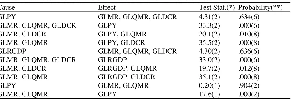
there is sufficient evidence that the financial variables cause the income variables.

However, there is less evidence of the reverse causality. For Korea, there is more

evidence that income variables cause the financial variables. There is much less evidence

in the reverse direction. Thus, Korea’s results are exactly the opposite of Japan’s. For

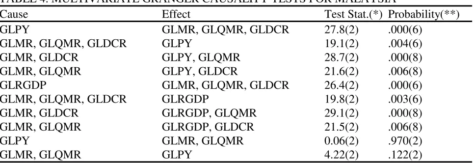
Malaysia, the results are similar to that of India in that we find evidence of a two-way

causality between the income variables and the financial variables. For Pakistan, per

capita income variable (GLPY) is found to be causing the financial variable but not vice

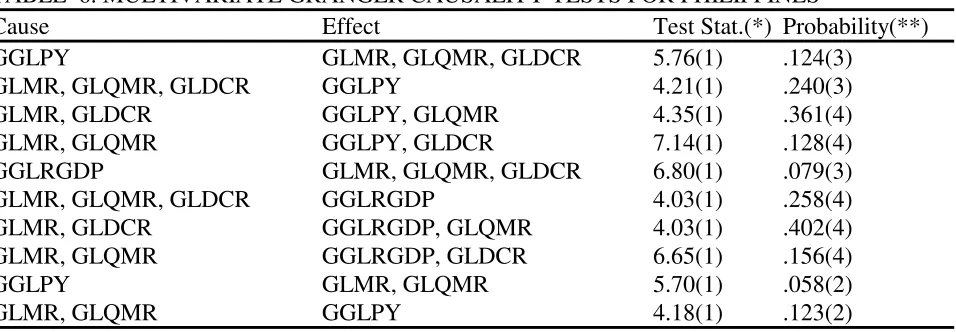
versa. For Philippines, there is some evidence that the GGLPY (the growth rate of

GLPY) causes GLMR (money supply variable) and GLQMR (quasi-money supply

variable). However, causality does not flow in any direction in any of the other cases.

For Sri Lanka, there is hardly any evidence of causality in any direction. For Thailand,

there is some evidence that the causality flows from the financial variables to the income

(15)

4. Conclusion

First, the empirical results from our study do not support the general consensus view of a

positive relationship between financial development and economic growth. The results

show a positive and significant relationship between the income and financial variables

for India, Malaysia, Pakistan and Sri Lanka. Second, the multivariate causality empirical

results are mixed. For India and Malaysia the evidence suggests a two-way relationship

between the income and financial variables. The results for Japan and Thailand suggests

a one-way relationship from financial variables to economic growth, while for Korea,

Pakistan and the Philippines, the results show the reverse causality. For Sri Lanka there

is little evidence of causality in either direction.

Therefore, an important implication that we can deduce from the empirical

analysis is that we cannot generalize about the relationship or the direction of causality

between financial development and economic growth, as quite a number of cross section

(16)

REFERENCES:

Ahmed, Syed-M and Ansari, Mohammed I (1998), “Financial Sector Development and Economic Growth: The South-Asian Experience.” Journal of Asian Economics, 9(3), pp. 503-17.

Ahmed, Syed-M and Ansari, Mohammed I (1995), “Financial Development in

Bangladesh- A Test of the McKinnon-Shaw Model.” Canadian Journal of Development Studies, 16(2), pp. 291-302.

Bagehot, Walter (1873), Lombard Street. Homewood, IL: Irwin.

Bencivenga, Valerie R and Smith, Bruce D. (1991), “Financial Intermediation and EndogenousGrowth.” Review of Economic Studies, 58(2), pp. 195-209.

Berthelemy, Jean-Claude and Varoudakis, Aristomene (1996),“Economic Growth, Convergence Clubs, and the Role of Financial Development.” Oxford Economic Papers, 48(2), pp. 300-328.

Berthelemy, Jean- Claude and Varoudakis, Aristomene (1998), “Financial Development, Financial Reforms and Growth: A Panel Data Approach.” Revue-Economique, 49(1), pp. 195-206.

De La Fuente, Angel and Marin, Jose Marias (1994), “Innovation, Bank Monitoring and Endogenous Financial Development.” Universitat Pompeu Fabra Working Paper, No.59.

Demetriades, Panicos and Hussein, Khaled (1996), “Does Financial Development Cause Economic Growth? Time Series Evidence from Sixteen Countries.” Journal of

Development Economics, 51(2), pp. 387-411.

Demetriades, Panicos and Luintel, Kul B (1996), “Financial Development, Economic Growth and Banking Sector Controls: Evidence from India.” Economic Journal,

106(435), pp. 359-74.

Dickey, David A and Fuller, Wayne A (1979), “Distributions of the Estimators for Autoregressive Time Series with a Unit Root.” Journal of the American Statistical Association, 74(Part I), pp. 427-31.

Dickey, David A and Fuller, Wayne A (1981), “Likelihood Ratio Statistics for Autoregressive Time Series with a Unit Root.” Econometrica, 49(4), pp. 1057-72.

(17)

Galbis, Vicente (1977), “Financial Intermediation and Economic Growth in Less

Developed Countries:A Theoretical Approach.” Journal of Development Studies, 13(2), pp. 58-72.

Goldsmith, Raymond W (1969), Financial Structure and Development. New Haven, CT: Yale University Press.

Granger, Clive W. J (1969), “Investigating Causal Relations by Econometric Models and Cross Spectral Methods.” Econometrica, 37(3), pp. 424-38.

Greenwood, Jeremy and Jovanovic, Boyan (1990), “Financial Development Growth, and the Distribution of Income.” Journal of Political Economy, 98(5, Pt.1), pp. 1076-1107.

Greenwood, Jeremy and Smith, Bruce D (1997),“Financial Markets in Development, and the Development of Financial Markets.” Journal of Economic Dynamics and Control,

21(1), pp. 145-81.

Gupta, Kanhaya L (1984),Finance and Economic Growth in Developing Countries, London: Croom Helm.

Gurley, John G., and Shaw, E.S (1955), “Financial Aspects of Economic of Economic Development.” American Economic Review, 45(4), pp. 515-38.

Hicks, John (1969), A Theory of Economic History, Oxford: Clarendon Press.

International Monetary Fund (1998) International Financial Statistics, CD-ROM version, November 1998.

Jayaratne, Jith and Strahan, Phillip (1996), “The Finance-Growth Nexus: Evidence from Bank Branch Deregulation.” Quarterly Journal of Economics, 111(3), pp. 639-670.

Jung, Woo S (1986), “Financial Development and Economic Growth: International Evidence.” Economic Development and Cultural Change, 34(2), pp. 333-46.

Khan, Ashfaque H and Hasan, Lubna (1998), “Financial Liberalization, Savings, and Economic Development in Pakistan.” Economic Development and Cultural Change,

46(3), pp. 581-597.

King, Robert G and Levine, Ross (1993a), “Finance and Growth: Schumpeter Might Be Right.” Quarterly Journal of Economics, 108(3), pp. 717-37.

(18)

Kwan, Andy C., Wu, Yangru and Zhang, Junxi (1998), “An Exogeneity Analysis of Financial Deepening and Economic Growth: Evidence from Hong Kong, South Korea and Taiwan.” Journal of International Trade and Economic Development, 7(3), pp. 339-54.

Levine, Ross (1997), “Financial Development and Economic Growth: Views and Agenda.” Journal of Economic Literature, 35(2), pp. 688-726.

Levine, Ross (1998), “The Legal Environment, Banks, and the Long-Run Economic Growth.” Journal of Money Credit and Banking, 30(3), pp. 596-613.

Levine, Ross and Zervos, Sara (1998), “Stock Markets, Banks and Economic Growth.”

American Economic Review, 88(3), pp. 537-558.

Lucas , Robert E (1988),“On the Mechanics of Economic Development.” Journal of Monetary Economics, 22(1), pp. 3-42.

Mathieson, Donald J (1980), “Financial Reform and Stabilization Policy in a Developing Economy.” Journal of Development Economics, 7(3), pp. 359-395.

McKinnon, Ronald I (1973), Money and Capital in Economic Development. Washington, DC: Brookings Institution.

Okedokun, M.O (1998), “Financial Intermediation and Economic Growth in Developing Countries.” Journal of Economic Studies, 25(3), pp. 203-234.

Patrick, Hugh T (1966), “Financial Development and Economic Growth in

Underdeveloped Countries.” Economic Development and Cultural Change, 14(2), pp. 174-187.

Porter, Richard C (1966), “The Promotion of the Banking Habit and Economic Development.” Journal of Development Studies, 2(4), pp. 346-366.

Rajan, Raghuram G. and Zingales, Luigi (1998), “Financial Dependence and Growth.”

American Economic Review, 88(3), pp. 559-586.

Ram, Rati (1999), “Financial Development and Economic Growth: Additional Evidence.”

Journal of Development Studies, 35(4), pp. 164-174.

Robinson, Joan (1952), “The Generalization of the General Theory.” in The Rate of Interest, and Other Essays. London: Macmillan, pp. 67-142.

(19)

Rousseau, Peter and Wachtel, Paul (1998) “Financial Intermediation and Economic Performance: Historical Evidence from Five Industrialized Countries.” Journal of Money Credit and Banking, 30(4), pp. 657-678.

Schumpeter, Joseph A. (1912), Theorie der Wirtschaftlichen Entwicklung [The Theory of Economic Development]. Leipzig: Dunker & Humblot, translated by Redvers Opie. Cambridge, MA: Harvard University Press, 1934.

Shaw, Edward S (1973), Financial Deepening in Economic Development. New York: Oxford University Press.

Singh, Ajit and Weisse, Bruce A (1998),“Emerging Stock Markets, Portfolio Capital Flows and Long-Term Economic Growth: Micro and Macroeconomic Perspectives.”

World Development, 26(4), pp. 607-22.

Spears, Annie (1992), “The Role of Financial Intermediation in Economic Growth in Sub-Saharan Africa.” Canadian Journal of Development Studies, 13(3), pp. 361-380.

Thornton, John (1996), “Financial Deepening and Economic Growth in Developing Economies.” Applied Economic Letters, 3(4), pp. 243-46.

Wachtel, Paul and Rousseau, Peter (1995), “Financial Intermediation and Economic Growth: A Historical Comparison of the United States, United Kingdom, and Canada”, in Michael D. Bordo and Richard Sylla (Eds.) Anglo-American Financial Systems:

(20)

[image:20.612.92.575.97.258.2]

TABLE 1. MULTIVARIATE GRANGER CAUSALITY TESTS FOR INDIA

Cause Effect Test Stat.(*) Probability(**) GLPY GLMR, GLQMR, GLDCR 30.7(2) .000(6)

GLMR, GLQMR, GLDCR GLPY 21.7(2) .001(6) GLMR, GLDCR GLPY, GLQMR 39.8(2) .000(8) GLMR, GLQMR GLPY, GLDCR 47.0(2) .000(8) GLRGDP GLMR, GLQMR, GLDCR 30.0(2) .000(6) GLMR, GLQMR, GLDCR GLRGDP 11.2(2) .083(6) GLMR, GLDCR GLRGDP, GLQMR 40.4(2) .000(8) GLMR, GLQMR GLRGDP, GLDCR 41.0(2) .000(8) GLPY GLMR, GLQMR 14.9(2) .005(4) GLMR, GLQMR GLPY 16.6(2) .002(4)

Note: The test statistic indicates the chi-square value. The probability refers to the probability of accepting the null hypothesis of no causality.

*indicates the number of lags which was determined by using the Akaike Information Criterion (AIC). **indicates the degrees of freedom of the chi-square.

TABLE 2 . MULTIVARIATE GRANGER CAUSALITY TESTS FOR JAPAN

[image:20.612.95.573.359.524.2]

(21)

[image:21.612.93.569.84.247.2]

TABLE 3 . MULTIVARIATE GRANGER CAUSALITY TESTS FOR KOREA

TABLE 4. MULTIVARIATE GRANGER CAUSALITY TESTS FOR MALAYSIA

[image:21.612.91.575.345.511.2]

(22)

[image:22.612.93.571.83.247.2]

TABLE 5 . MULTIVARIATE GRANGER CAUSALITY TESTS FOR PAKISTAN

Cause Effect Test Stat.(*) Probability(**) GLPY GLMR, GLQMR, GLDCR 21.4(2) .002(60

TABLE 6. MULTIVARIATE GRANGER CAUSALITY TESTS FOR PHILIPPINES

Cause Effect Test Stat.(*) Probability(**) GGLPY GLMR, GLQMR, GLDCR 5.76(1) .124(3)

GLMR, GLQMR, GLDCR GGLPY 4.21(1) .240(3) GLMR, GLDCR GGLPY, GLQMR 4.35(1) .361(4) GLMR, GLQMR GGLPY, GLDCR 7.14(1) .128(4) GGLRGDP GLMR, GLQMR, GLDCR 6.80(1) .079(3) GLMR, GLQMR, GLDCR GGLRGDP 4.03(1) .258(4) GLMR, GLDCR GGLRGDP, GLQMR 4.03(1) .402(4) GLMR, GLQMR GGLRGDP, GLDCR 6.65(1) .156(4) GGLPY GLMR, GLQMR 5.70(1) .058(2) GLMR, GLQMR GGLPY 4.18(1) .123(2)

Note: The test statistic indicates the chi-square value. The probability refers to the probability of accepting the null hypothesis of no causality. GGLPY and GGLRGDP stand for the first differences of GLPY and GLRGRDP respectively.

[image:22.612.95.573.332.498.2]

(23)

[image:23.612.92.575.97.261.2]

TABLE 7. MULTIVARIATE GRANGER CAUSALITY TESTS FOR SRI LANKA

TABLE 8. MULTIVARIATE GRANGER CAUSALITY TESTS FOR THAILAND

Cause Effect Test Stat.(*) Probability(**) GGLPY GLMR, GLQMR, GLDCR 0.99(1) .803(3)

GLMR, GLQMR, GLDCR GGLPY 6.63(1) .085(3) GLMR, GLDCR GGLPY, GLQMR 10.9(1) .028(4) GLMR, GLQMR GGLPY, GLDCR 7.11(1) .130(4) GLRGDP GLMR, GLQMR, GLDCR 1.22(1) .748(3) GLMR, GLQMR, GLDCR GLRGDP 3.69(1) .297(3) GLMR, GLDCR GLRGDP, GLQMR 5.30(1) .258(4) GLMR, GLQMR GLRGDP, GLDCR 8.13(1) .087(4) GGLPY GLMR, GLQMR 1.48(1) .478(2) GLMR, GLQMR GGLPY 5.58(1) .062(2)

Note: The test statistic indicates the chi-square value. The probability refers to the probability of accepting the null hypothesis of no causality. GGLPY stands for the first difference of GLPY.

[image:23.612.91.573.360.525.2]