Munich Personal RePEc Archive
Barter relationships
Prendergast, Canice and Stole, Lars
University of Chicago Booth School of Business
January 2000
Barter Relationships
∗
Canice Prendergast
†Lars Stole
‡January 2000
Abstract
We offer a simple economic model of repeated barter to explore current economic
exchange in Russia: individuals trade with each other in a dynamic environment where
the threat of dissolving the relationship constrains the incentives to cheat. We show
how the value of future interactions affects the willingness of individuals to trade with
each other; only when rates of interaction are large can trust compensate for an absence
of money. Moreover, when trading relationships are asymmetric – either in the trading
partners’ values for each other’s goods or in their relative bargaining power – the
resulting barter allocations are distorted, as goods must be used for liquidity reasons.
When third-party middlemen exist who can facilitate barter, they command a premium
for their services, and have preferences for improved liquidity which may or may not
correspond with the other traders in the barter economy. Fourth, we demonstrate that
the restriction of trading to tight trading networks may be a socially efficient response
to insufficient barter interactions. Finally, we consider how liquidity constraints affect
pricing, and illustrate how the existence of a barter market can mute incentives to
change prices in response to credit crunches.
∗Published as Chapter 2 inThe Vanishing Rouble: Barter Networks and Non-Monetary Transactions in
Post-Soviet Societies, Paul Seabright, editor, Cambridge University Press, 2000.
†University of Chicago, GSB & NBER
‡University of Chicago, GSB and Research Fellow, CESifo. We are grateful to Paul Seabright and
1
Introduction
Economists interested in barter and non-monetary exchange often talk at cross-purposes to
anthro-pologists and sociologists. Central to the anthropological literature is the notion of delayed
reci-procity, where barter deals “require delays in payment and several exchanges before the transactors
are satisfied” (Humphrey (1998)). This observation has been a central theme in the anthropology
of exchange since Mauss (1990[1950]) and Malinowski (1961), and an important component of this
research has focussed on the realization that such exchange requires institutions that persuade
peo-ple to reciprocate favours. However, traditional monetary economics has largely dealt with cases
in which such enforcement issues are absent, either by assuming simultaneous barter or
enforce-able long-term borrowing and lending contracts. Missing from this literature is the importance of
implicit arrangements which are based on trust.1 The purpose of this paper is to redress this
some-what, relying on a large, recent literature on self-enforcing contracts, which often examines trade
where money is absent. We argue that useful insights on barter can be obtained by using an
eco-nomic analysis of repeated exchange with little or no money or external enforcement mechanisms,
but where trust plays a central role.
This chapter is not meant to provide a holistic view of non-monetary social exchange in general,
which involves an array of moral, religious, cultural, and economic aspects. Instead, its objective
is to address some aspects of repeated exchange which operate in the wild economic environment
of Russia.2 It considers the operation of agents (firms or individuals) in an “economy of favours”
(Ledeneva, 1998a), each of whose objective in exchange is to maximize their own economic return
subject to whatever social, institutional, or implicit constraints that they and their trading partners
face. Given the breakdown of social commitments and moral obligations which characterize the
descriptions of Russian exchange in this volume, we believe that the tools of economics can provide
a useful framework for understanding some phenomena.3
Throughout the paper, we borrow liberally from recent advances in the economic literature
on repeated game theory which studies environments in which there is little external enforcement
of contracts, but where the individuals themselves must design informal institutions to manage
1
For example, Lemon (1998) cites economists as “believing barter to be the extreme case in which no trust is present in the system.”
2
As described in this volume, the environment of exchange is characterized by “pride in acquiring” rather than giving (Humphrey, (1998)), replete with opportunities for “cheating, defaulting and illegalities” and where there are “no longer pregiven social commitments” (Anderson (1998)). These aspects will be features of the economic model we offer below.
3
trade.4 With some notable exceptions such as Kranton (1996, 1998), there have been few attempts
to understand barter arrangements from this perspective – a perspective which recognizes the delay
and trust which is inherent in barter exchange. We have also tried to minimize as much as possible
the technical difficulties of the paper. For those interested in a more technical treatment of some
of these issues, see our companion papers (Prendergast and Stole, (1998a, 1998b, 1998c)). In cases
where some technical details are required, they are largely relegated to an Appendix to render the
paper more readable.
A number of themes run throughout this paper. The first theme which we emphasize is the costs
of barter relative to a monetized economy. This is a central concern of classical monetary theory
which emphasizes reductions in trade which arise because there is an absence of a static double
coincidence of wants.5 Money, because of its commonly accepted value, provides for this double
coincidence. We leave such inefficiencies largely in the background and instead emphasize a series
of more subtle and less studied issues. First, we begin with the most basic model of reciprocated
exchange in Section 2, where two individuals would like to trade with each other over time, but do
not have money to facilitate exchange. The individuals are symmetric in that they value each other’s
good equally and with similar frequency, though (importantly) their demands are not simultaneous.
In this simple setting, we illustrate the ability of the individuals to reciprocate trade when the
penalty for failing to do so is the dissolution of the relationship, a common enforcement mechanism
in many societies (see Sahlins (1972) on this).6 In our simple benchmark model with similar
traders, the ability to trade depends on the importance of the relationship, namely, the frequency
of interaction and the patience of the individuals, where traders compare the benefits of reneging
on the relationship with the lost surplus that would ensue if they did.
The purpose of section 2 is simply to illustrate how the modern tools of economics can aid
in our analysis of the decisions taken by agents and the resulting levels of trade.7 The simple
economic model we present, while useful in developing an understanding of the importance of
future interactions, is limited in that there are many dimensions on which the model fails to capture
important aspects of observed exchange. Recognizing these limitations, we proceed through the
4
For those interested in learning more about this literature, we recommend a textbook by Fudenberg and Tirole (1991). For early work on self-enforcing contracts, see Telser (1980) and Klein and Leffler (1981).
5
To take a trivial example, if you only have broccoli to trade for my coffee, and I don’t like broccoli and can’t easily trade it on to someone else, the trade is unlikely to be consummated.
6
In this sense, we differ little from Firth’s (1939) observation on the Maori that “the main emphasis of the fulfillment of obligation lies..[in] the desire to continue useful economic relations” (page 421).
7
remaining sections of the paper by introducing variations into our framework to explore these
additional issues.
In section 3 we adapt our model of repeated exchange to deal with the fact that one agent may
need the good of this trading partner more than vice versa, or one agent may be more “powerful”
than the other. In this section, we demonstrate a second theme: such asymmetries can cause
additional barter inefficiencies through different outcomes than those which would occur in an
exchange environment mediated with money. For example, when individuals find it difficult to
enforce trade through reciprocal exchange, production of “unwanted” goods is typically higher
than those which are in greater demand, in sharp contrast to the outcome of a monetized economy.
The reason for this is that these unwanted goods serve, in part, the role of currency and one may
find “liquidity” value in them as a means of exchange. We also relate the resulting outcomes to
discussions of pricing in other chapters of this volume, where we show how the terms of trade offered
to those with “unwanted” goods depends on the trading relationship. Specifically, the price paid
for valued goods (in terms of “unwanted” goods) gets worse as relationships become less important.
Another recurring theme of the papers included in this volume is the importance of networks
for facilitating trade. Section 4 analyzes a simple network to illustrate some issues which appear
relevant to the Russian experience. Foremost among these issues is an understanding of the
distri-butional implications of barter exchange in Russia, a third theme of the paper. It seems clear from
the work presented by Alaina Lemon (1998), Alena Ledeneva (1998b), Caroline Humphrey (1998)
and David Anderson (1998) that transacting through personal contracts does not lead to a level
playing field. One can think of established network links as a scarce economic resource which takes
time to develop, and whose presence tilts economic power towards the linked trading partners. In
particular, established firms, often those from the Soviet era, appear to be in a particularly good
position due to both the volume of trade that they are involved in and the central position that they
hold in production networks. These are the “good old” contacts described by Ledeneva (1998b). By
contrast, some firms and individuals appear to have been left behind in this world of contacts, not
least the Roma described by Lemon (1998). An additional implication of this, modeled in Section
4, is the demand which this generates for middlemen, who appear to play a central role in many of
the network discussions in this volume. However, these middlemen typically take advantage of their
position in the networks and extract some of the surplus from the trade based on whatever they
can contribute to the exchange. This section also points to an additional distributional implication
of the barter economy, namely, that there are likely some individuals which have benefited from
the demonetization of the country, largely as it increases the value of their advantaged position in
A fourth theme which we address is how individuals choose to construct their networks. Many
sociologists take a rather structuralist approach to networks (see Burt (1992), for example), where
networks are simply assigned, even though it frequently appears to be the case that individuals
explicitly and strategically create networks. In Section 5 we consider an additional aspect of
networks in that when money is absent, it induces individuals to have concentrated networks,
rather than relying on many producers who may be able to produce at lower cost. An implication
is that individuals will sometimes forego the benefits of comparative advantage in order to keep a
relationship going. The reason for such a policy of “putting all your eggs in one basket” is that it
tends to increase incentives for trustworthy dealings compared to a situations where one’s partner
is of little importance. A related implication of this contribution is that in barter settings, it may
be difficult to break into a trading network, even in cases where a producer has something of value
to another.
Finally, in Section 6, we consider how barter markets can interact with cash markets.
Specif-ically, we consider a world characterized by liquidity shocks, where individuals simply may not
have enough money to buy their preferred goods. We are particularly interested in the effect of
barter and liquidity shocks on prices. We assume that liquidity shocks are not common across all
people in the economy: instead, they differentially affect people with low valuations more than
those with high valuations. For example, people with low income are less likely to purchase certain
goods at any given prices, even without a liquidity shock, and so it is these people who are most
affected by such a shock. Using this assumption, we show three main effects of a liquidity shock on
prices. First, if the liquidity shock is large enough, prices will fall below those which arise without a
liquidity shock. This supports our usual notion that demands for money are tempered in a setting
where there is little money. However, our second finding is that, again if the liquidity shocks are
large enough, the reduction in prices caused by liquidity shocks is muted when sellers can also
barter their goods. In other words, the opportunity to barter stops prices from falling as much as
they would otherwise. As a result, the barter market constrains price reductions from a liquidity
shock. Third, for less severe liquidity shocks, we show that prices will be above those without a
liquidity shock, a result which arises either with or without the opportunity to barter. But the
price movements induced by liquidity shocks are nonetheless more muted in the presence of barter.
In other words, barter has the effect of reducing cash-price flexibility in response to shocks, as
the barter markets provide an effective alternative to the cash market and become relatively more
2
A Simple Model of Reciprocal Barter
We begin by considering the simplest possible setting of repeated exchange, where two symmetric
individuals with equal bargaining power interact to supply goods to each other. To do so, we set up
a stylized “repeated game,” in which two individuals trade with each other, but where the only way
to reward a trade partner is by offering a good in the future; there is no money to satisfy a static
double coincidence of wants. Periodically, each party demands goods from the other, and the other
must make a voluntary choice whether to provide those goods. The individuals interact repeatedly
so that one partner can use the threat of terminating the relationship as a way of persuading the
other partner to supply goods to them. As a result, agents weigh the personal gain from continuing
the relationship and supplying goods to the other at some immediate cost against violating the
implicit duty to supply which would end the relationship. In this setting, not surprisingly, the
importance of the future relationship to the individuals plays a critical role, with trade being easier
to enforce when the relationship has dense or highly valuable future trading opportunities than
when trade is sporadic or of low value.
The formal model we offer requires some notation but is logically straightforward. In keeping
with the specifics of much of Russian barter, we assume an absence of a double coincidence of
wants; instead there is some delay between exchanges so that the individuals must reciprocate
goods and favours to each other over time. Consider two individuals who interact over time,
potentially providing goods to one another other whenever called upon to do so. Each party to the
relationship has a good which their partner may demand in any period of time. To be specific, we
assume that when a good is demanded by individual A and q units are supplied by individualB,
a value ofq accrues to agentA at a cost of c(q) = 12q2i which is borne by individualB; the reverse
is true when the demand is made by individualB. We can then definev(q)≡q−c(q) as the joint
surplus created from the trade of the good. Importantly, agents cannot satisfy their own needs.
We consider the arrival of demands (which we sometimes refer to as projects) to be a random
process with a project for person i arriving during a short period of time, ∆, with probability
λ∆; i.e., projects arrive according to a Poisson process. This seemingly complicated dynamic
process is in fact extremely simple to deal with, as we will see below. With this description of the
availability of productive projects, we can think of a higher λ as corresponding to more frequent
trading opportunities. Indeed, simple statistical calculations verify that 1λ represents the average
time between opportunities. Another attraction of thinking about projects arriving randomly over
time according to our λdistribution is that that a doublestatic coincidence of wants occurs with
insignificant probability; as a result, reciprocal exchange over time is the only possible avenue for
Visually, the trading network can be illustrated as in 1.
Figure 1: Bilateral Exchange
B
A
goods exchanged bilaterally
Recall that 1λ represents the average time between trading opportunities. The time between
trades is relevant as people are impatient: Everything else equal, consumption today is better
than consumption next year, and production today is more costly than production next year. We
model this impatience by assuming that individuals have a subjective discount rate which can be
thought of as an internal rate of interest; we denote this rate with the notationr. Mathematically,
it will be the case that the ratio of the interaction rate to the value of that time, λ/r, will be the
critical determinant for whether or not cooperative trade is sustainable. This ratio is a measure
of the relative frequency of trade. A higher ratio implies that the expected present value gains
from ongoing trade is higher, and hence we will see that cooperation through dynamic reciprocity
is easier to sustain. Lower values of this ratio indicate that the relationship is more transient with
only sporadic interaction.
To see the role of this ratio more precisely, consider trade in this environment where there is
potentially reciprocated exchange. Here, the agents enforce reciprocal trades through the threat of
dissolution of the partnership.8 We initially consider symmetric solutions to this problem, where
each agent receives the same quantity ofq from the other.9 Then if one agent requiresq, the other
agent is willing to provide it only if
V(q)≥c(q), (1)
where V(q) ≡ λ
r[v(q)] represents the expected return of the indefinitely recurring relationship to
a trader. Therefore, V(q) is the value of the relationship. Note the importance of the λr term: a
higher ratio directly implies a higher value to the relationship.
The requirement for cooperation in the incentive equation above forms the foundation for this
paper so it deserves some elaboration. The person who is called upon to produce has a choice;
either produce the good, which costsc(q) or renege, in which case no costs are incurred. All other
8
“We know what happens when a trade partner is disinclined to reciprocate - the sanction everywhere is dissolution of the partnership” (Sahlins (1972), p. 312).
9
things equal, the person would prefer not to incur this cost. However, if she fails to produce, she
has reneged on the relationship and loses the future value of that relationship, which is V(q), as
the relationship is dissolved. Therefore only if V(q)−c(q) ≥ 0 will she actually carry out her
obligations.
The next step in solving this problem is in understanding how much trade individuals will be
willing to fulfill. If each party could pay for the goods in a commonly accepted currency, the
quantity traded would be qef f = 1 – this is the “efficient” level of trade which maximizes the
relationship’s value,V(q). However, our agents do not have money and must rely on the reciprocal
exchange of favours. They choose the maximum level of q (up to the efficient level of 1) that the
provider of the good is willing to offer. The trades can be characterized by two regions. For large
enough λr, the incentive constraint (1) does not bind at the efficient level of trade, qef f = 1, so
they will produce efficiently. In other words, if agents interact frequently, or the surplus is large
enough, trade is efficient and the absence of money is overcome by the existence of repeated
ex-change. In more colloquial terms, trust can substitute for cash. For lower rates of interaction,
both quantities are below the efficient level, as the value of the relationship does not make
produc-ing higher output worthwhile. Note that the quantities of both goods continuously increase in λr
so that as the relationship becomes more important, quantities rise to the surplus maximizing levels.
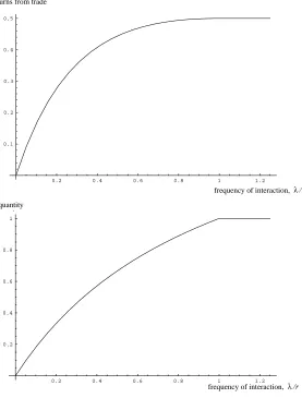
Example 1: For an illustrative case consider the setting in Figure 2. The curve in the top
graph gives the (maximal) flow value from the relationship rV(q) as a function of the frequency of
interaction (normalized by the cost of time) λ
r. This is the total surplus generated for each party.
Figure 2. The Effect of Interaction Frequency on Dynamic Reciprocity
quantity
λ
frequency of interaction, /r
returns from trade
0.2 0.4 0.6 0.8 1 1.2
0.1 0.2 0.3 0.4 0.5
0.2 0.4 0.6 0.8 1 1.2
0.2 0.4 0.6 0.8 1
λ
frequency of interaction, /r
Figure 2 illustrates the importance of λr for trade, with quantities traded increasing in the
frequency of interaction, up to the point of efficient trade, beyond which there is no reason to
increase trade further. This section demonstrates the importance of repeated interaction in effecting
barter exchange. If money were freely available, there would be no reason for repeated exchange.
With money absent, the threat of dissolution acts to constrain cheating, and so it is important that
the agents value the relationship in order to act honestly.10 This section therefore illustrates one
cost to barter exchange in repeated settings, namely, that individuals are sometimes focused on
short term gains so much that they renege on their reciprocal obligations. (Or to phrase it another
10
In one sense, this section is little more than a formal illustration of the schema of reciprocity offered by Sahlins (1972). He characterizes different types of reciprocity based on the distance of a trade partner from the individual. At the top of this hierarchy is generalized reciprocity, where high levels of trade are possible with members of one’s own kinship groups. At the other extreme is the negative reciprocity offered to strangers, where an individual will happily harm the person he is trading with. This model describes distances in terms of λ
way, as individuals value relationships less and less, smaller quantities of trade can be supported.)
There is much evidence to suggest that such inefficiencies arise. First, many of the contributors
to this volume cite the wild nature of the Russian economy where incentives to default prevail,
while Ledeneva (1998b) also emphasizes the critical importance of “good old” personal contacts for
ensuring that trade actually happens.
3
Inefficient, Delayed Rewards and the Liquidity Value of Trade
This section deals with cases where one agent’s goods are of higher value that those provided by
the other. Put simply, how does reciprocity operate in situations where one agent demands more
from the other than vice versa? So far, we have offered one reason why economic relationships
without money can be inefficient: trade is not frequent enough (or, alternatively stated, individuals
are not sufficiently patient). However, there are other problems which can arise when money is
absent, many of which related to inherent asymmetries between the two parties. (Remember that
in the previous section, we have assumed that the two parties value each other’s goods equally.) A
recurring theme on barter in this volume is that many of the goods traded are not so desirable to one
of the parties, and may take time and involve other costs to offload. Equally there are cases where
one party needs things frequently from the other, while the reciprocal demands from the other
party are much more intermittent. There is furthermore considerable evidence from these papers
that the terms of trade depend on what currency is bartered, which this section also addresses.
When individuals value each other’s contributions differently, two additional insights arise.
First, agents trade with one another not simply for the consumption value of trade but also to
provide “liquidity,” serving a role as a quid pro quo for the exchange.11 The role of commodities
as a form of money gives rise to qualitatively different outcomes than those which arise in a
mon-etized economy. Second, pricing depends on both the goods traded and on the importance of the
relationship, where low-value goods and goods in sporadic relationships may receive poorer terms
of trade relative to high quality goods.
3.1 Asymmetric Values in Trading Relationships
In order for such liquidity provision to play a role, we first consider asymmetries between the agents,
where one agent values a unit of consumption of the other’s good more than vice versa. To this end,
we extend our basic model of Section 2 by assuming that one individual, person A, values a unit
of the other agent’s good at αq, where α >1. We call this high-valuation consumerthe α-agent.
11
The other individual,B, continues to have unit marginal utility for consumption. Note that higher
optimal production,q =α >1, is called for when serving theα-agent, relative to the other agent for
whom optimal production remains at 1. These are the outcomes of a monetized economy. However,
to induce the other person to offer higher quantities of the α-good in a barter setting, the agent
must offer something in return. In the absence of money, this becomes the other good, so that
production decisions will be partly determined by the desire to satisfy the other agent’s demands
at the higher level of production. In this sense, production decisions will be partly determined by a
wish to create a dynamic double coincidence of wants, as there is no static coincidence of wants.12
The lower-quality good has a “liquidity” orquid-pro-quovalue in a barter exchange which accounts
for why it is over-traded relative to the allocation in a monetary economy.
Our interest here is in identifying the quantities of goods which the individuals are willing to
trade. In order to render the paper more readable, we relegate much of the technical detail to the
Appendix of the paper, where a more formal proof of the propositions is offered. Verbally, the
quantities traded have the following characteristics. First, if the agents do not interact frequently,
trade is below its efficient level, and trade of the low-value good exceeds that of the superior
good. Ironically, the worse is the low-value good relative to the superior, the greater is its relative
production. For intermediate rates of interaction, trade in the low-value good is below that of
the superior good, but higher than the efficient level which would arise if money were available.
Finally, if the individuals interact frequently enough, there is no difference between the outcomes
with barter and with money.13
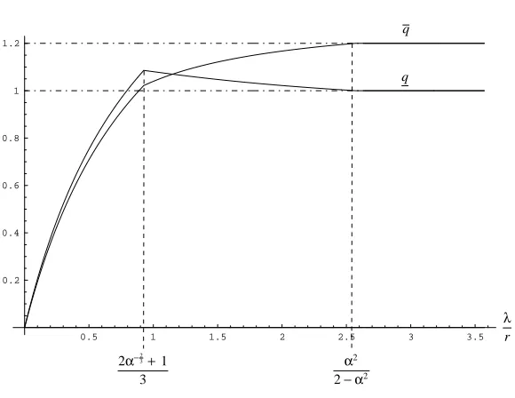
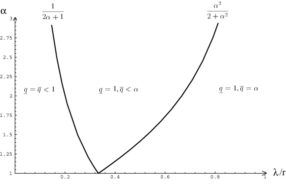
A visual characterization of the solution is given in Figure 3, where q is the production of the
superiorα-good and q is the production of the lower-valued good. In this example, we setα= 1.2.
12
Throughout this section, we simply maximize the sum of utilities. An interpretation of this is that each agent is
ex anteidentical, where nature determines which agent is theα-agent. Decisions on the equilibrium are taken before the draw from nature, so all agents agree on the objective function.
13
Figure 3: Liquidity and Trade
3 1 2α−32+
α − α
2 2
2
λ
r q
q
0.5 1 1.5 2 2.5 3 3.5
0.2 0.4 0.6 0.8 1 1.2
Remember that if money was freely available, the outcomes would beq=αandq= 1 regardless
of the rate of interaction, λr. Such efficient levels only emerge under dynamic reciprocity if the
rate of interaction is high enough; again, if the relationship is sufficiently important, trust can
substitute for cash. More generally, though, from Figure 3 one can see that there are three separate
regions. The one that seems of most relevance to the examples cited for Russia concern those
where interaction is infrequent (λr low). This is the part where both lines are upward sloping. For
example, Humphrey (1998) cites the “short horizons” of many barter participants. Note that when
interaction is infrequent, production of the worse good q is higher than production of the better
good and liquidity concerns reverse our normal intuition on the supply of goods, where goods with
higher marginal valuations have higher production.14
We can easily rephrase these results in terms of pricing behavior: in relationships where
inter-action in infrequent, those with poor barter goods get bad prices. In order to consume something
that they like, those with poor barter goods generally pay a dear price, sometimes having to
pro-duce large quantities to get anything in return. This appears to correspond to a recurring theme
in many of the papers offered in this volume. For example, Anderson (1998) describes the
“ex-ploitative side” of these trades, with barter prices being “more expensive than purchasing goods at
14
It is worth briefly noting the two other regions of trade here, though it is not our primary focus. First, note that trade in the less desirable good declines in λ
r after some point. The reason for this is that in this region, as λ r
increases, the value of the relationship rises for all agents, thus reducing the need to oversupply the less useful asset. Thus increased patience reduces some trades. Finally, for large enough λ
r, the efficient allocation (i.e., the outcome
wholesale prices”. It is easy to translate our results into relevant prices: the price is the quantity
of one good which must be offered to get a unit of the other. Not surprisingly, as the difference
between the two goods’ qualities increases, more of the low-valued good must be offered to get a
unit of the better good; in effect, the price of the better good rises. From this perspective, it is
hardly surprising that the prices denominated in petrol would be better than those denominated in
electric energy which “is not an easy currency” and “produces big discounts” (Ledeneva (1998b)).
In essence, prices reflect the quality of the bartered goods.
Another implication of this simple model is that it shows how pricing varies by the importance
of the relationship. Figure 4 plots the price of theα-good denominated in terms of the other good
as λ
r changes. This represents the amount of the less desirable good which must be offered to get a
unit of the better good. It is immediately seen that the relationship is (weakly) downward sloping,
so that the cost of getting the better good falls as the relationship becomes more important. Also
note that in relationships which are more important, the terms of trade get closer to the efficient
level, with traded quantities similar to those which would emerge in a world with money.15 When
the relationship is unimportant, the price of getting the preferred good is highest and most out of
[image:14.612.127.489.426.624.2]line with the efficient price level. Thus pricing depends on relationships.
Figure 4: Pricing In Relationships
0.2 0.4 0.6 0.8 1 1.2
0.46 0.5 0.52 0.54
cash prices
pure-cash price cash price in tandem
with barter
liquidity shock, z
These observations illustrate how non-monetary exchange operates in a different fashion to
monetary exchange. For instance, it is one of the most basic premises of economics that goods
15
which have higher marginal surplus will have higher production than those which are less valuable.
But this basic premise is violated here where there is more production of the less useful good. In
addition, we have pointed out the poor terms of trade which arise when agents have goods which
have poor liquidity; those who pay in petrol generally do better than those paying in bricks.
3.2 Asymmetric Bargaining Power
So far, we have only considered those cases where bargaining power worked such that the sum of
individual utilities was maximized. Yet many of the papers in this volume focus on the advantaged
position of some agents relative to others, manifesting itself in terms of asymmetric bargaining
power. A central theme of recent contributions to economics concerns inefficiencies that can be
generated by bargaining distortions. Two cases are generally considered; those in which everyone
knows the other’s valuations and those where valuations are unknown. In this section, we consider
the simplest case, where two agents trade with known valuations but where there is asymmetric
bargaining power. In a set of related papers, we develop the effects of barter upon bargaining
distortions in environments of incomplete information.16
When money is freely available, such asymmetric bargaining power worries economists little, as
higher bargaining power results in a weak agent simply paying more money, with no change in the
efficiency of the allocation. There is only a pure distributional effect about which we have little to
say. However, this is not so in the case of barter; here asymmetric bargaining power directly affects
the efficiency of the allocation – judged relative to a monetary economy – as greater bargaining
power is now manifested in terms of inefficient distortion of goods. For example, a farmer in
Russia with little bargaining power may be required to hand over excessively large quantities of
food to a powerful buyer, who offers little in return. In a monetary economy in which both parties
had ample monetary assets, such bargaining power may result in large cash transfers, but not in
inefficient allocations of goods. Such distortions in production are the standard efficiency losses of
economics.17
In order to isolate the effect of bargaining powerper se, consider a case where agents interact so
often that the incentive constraints are irrelevant (in the context of the formal model, assume that
interaction is very high) and their demands are assumed to be symmetric, as in Section 2. Suppose
instead of simply assuming that the agents split the surplus, they bargain over the allocation.
Following work by Rubinstein (1982), a simple way of parameterizing bargaining power relates to
16
Prendergast and Stole (1998a, 1998c). 17
the patience of the individuals involved. In this case, those with weak bargaining power cannot
wait to consume the good, while those with stronger bargaining power are content to sit out some
time before consuming. Although trades in these models occur immediately, the terms of trade
benefit the more patient bargainer. Suppose initially that each party is equally patient. Then
the bargaining outcome offers q = 1, the same outcome as with money. (Remember that we are
restricting attention to the case where the agents have symmetric demands and interact frequently,
so that we do not have to worry about the problems of the previous subsection.) This merely
replicates our earlier results. However, the presence of asymmetric bargaining power will generate
differences between the two allocations. As an example, consider the case where agent A has all
the bargaining power, allowing her to make a take-it-or-leave-it offer to the her trading partner.
Then the barter allocation hasB’s consumption given byqB <1 and agentA’s consumption given
by qA>1.18 In other words, asymmetric bargaining powerper se causes problems, with the party
with more bargaining power getting quantities which are too high while his less patient partnership
consuming too little relative to a monetized economy.
4
Networks and Distributional Effects of Barter
Perhaps the dominant theme of the papers in this volume has been the importance of contacts and
networks in current economic exchange in Russia, and some of the more fascinating contributions
illustrate the quite incredible sophistication of the networks which sometimes develop to satisfy a
double coincidence of wants. Ledeneva’s (1998b) contribution here is particularly apposite. The
importance of this institution of exchange should not be underestimated in understanding how
barter affects modern Russia. First, as Anderson (1998) nicely puts it: “the logic behind market
economies is that commodities, such as money, are intended to bind together many diverse
com-munities of exchange. The recent financial crisis .. (has) disqualified the (new) ruble from the role
of an instrument of social integration”. Or to put it another way, one person’s money is as good as
another’s,19 so money facilitates exchange between individuals with little in common. By contrast,
one person’s social contacts clearly are not the equal of anothers.
This transition from an economy based on money to one based on contacts surely has important
effects on distribution and social integration. In terms of the simple model above, individuals
differ in terms of their trading intensities (i.e., λ/r), where those with less frequent interactions
become excluded from trades which would otherwise occur with money. There can be little doubt
from Lemon’s (1998) contribution that this has adversely affected the Roma, who are often seen
18
More precisely,qB= 2−
1
3 andqA= 2 1 3.
19
as untrustworthy by Russians. Equally, Humphrey (1998) notes that farmers are restricted to
simultaneous barter arrangements, as they lack the relationships to ensure delayed reciprocity. Yet
such exclusion is not restricted solely to particular ethnic or occupational groups. Instead, it is
clear that individuals seek out trade partners with good pedigrees, or at least pedigrees where there
is evidence of dense trade. As Anderson (1998) notes, there is a difficulty in building “networks of
alliance in a space where there are no longer pregiven social commitments.” For instance, Ledeneva
(1998b) emphasizes the importance of “good, old” contacts, while Humphrey notes the importance
of networks that are often “quite simply based on Soviet-era links,” where firms “prefer to work
with solid government-supported firms.” Clarke (1998) notes that two classes of contacts become
important:, those who “had their roots in old administrative structures” and “those outside the
law.”
These observations seem to point to the importance of established trade partners, those with
links to many other firms, which may be necessary to provide the ultimate “cash” of the barter
arrangement. Those with few links to other networks become poor trading partners, at least
in the absence of middlemen. It is our sense that this is of critical importance for the Russian
economy and perhaps political future. One implication of such barter networks is that they exclude
individuals on the periphery (the Roma being the extreme social example of this) and also give a
huge advantage to those who are already in established networks. It is not hard to see potential
implications for restructuring and government in Russia. Particularly, because of demonetization,
older established firms, often those which are the “dinosaurs” of Humphrey’s (1998) analysis, are
increasingly becoming central to economic exchange, despite the extinct nature of the outputs that
they produce. Since these firms often have strong contacts to local government, it is also not hard
to imagine a link to political entrenchment.
The importance of networks for facilitating trade has numerous implications. First, as described
above, it can exclude peripheral individuals from exchange. A second implication, which we briefly
model here, concerns the importance of middlemen to economic exchange. As Clarke (1998) notes,
“to find new customers and suppliers, enterprises had to turn to intermediaries, ... individuals who
had their own contacts and sources of finance”. To illustrate this, we consider a simple network
which requires a middleman to facilitate exchange. However, an additional purpose of this is to
note that the middleman does not come for free; positions in networks generate rents which reduce
the value of trade to the parties who are involved in production. Indeed, we will show below that
middlemen may actually benefit from the demonetization process: they are only needed when times
are sufficiently bad, and so (in some cases) may disappear when times get better.
some liquidity in the system, though the trading individuals cannot be assured of having enough.
To model this and the need for middlemen, we begin by extending the model of liquidity trade
above in Section 3 by assuming that another individual can provide liquidity. As noted above,
parties A and B may not interact enough to get to the same outcome as the monetized economy.
This is where middlemen play a role. They can in effect partially monetize the barter transaction
by providing transfers between the parties with some regularity. We model this simply here by
assuming that there is another party, C. This party fills a need betweenA andB in the following
way. We assume that A has a project withC where he can transfer a good to C. For simplicity
we ignore the productive value of the trades with C by assuming that transfers from A to C are
welfare neutral, where a transfer of goods costing xtoAhas valuex toC. In turn, C can transfer
something to B, where a transfer of goods costingx toC has value x toB. Thus C plays no role
other than to shuffle resources from A, the consumer of the superior good, to B the consumer of
the low-value good.20 Thus, when A wants something, B will provide it and gets (possibly) two
things in return: goods from A and and a transfer from C. These occur sometime in the future.
(Without the middleman,B can only obtain goods from A.) The role of party C, who acts like a
bank, is that it can transfer resources to B when available and required. To retain symmetry in
the model, we also assume that C receives each of his projects (the project from Abeing one, the
project to B being the other) with frequency µλ, where a higher value of µ is akin to increasing
the liquidity available to party C. As with the liquidity model of Section 3, agent A prefers the
good provided by B (with marginal utility α > 1) relatively more than B likes A’s good (which
has marginal utility of 1).
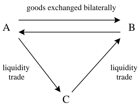
Visually, our network is given in Figure 5.
20
Figure 5: The Network With A Middleman
B
C
A
goods exchanged bilaterally
liquidity
trade
liquidity
trade
Of course, the agent providing liquidity will not do so for free; A must pay him. Since it
facilitates trade,Cwill demand a share of the increase in trade by threatening to abscond whenever
he is required to give something toB. Amust provide C with a credible promise of future returns
to prevent this behaviour. Thus, when A has an opportunity to transfer value to C via some
project, she will do so to the extent required. As with the previous sections, we assume that the
parties maximize the sum of their utilities, subject to the relevant incentive constraints of the type
described in Section 2.21 The main difference in the formal model is now that party C must be
induced to hand over a transfer toB when he is called upon to do so.22
As in the previous sections, we do not provide exhaustive details of our theoretical results.
Instead, we simply provide an example to illustrate the main implications of allowing middlemen.
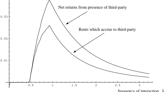
The outcome of the provision of liquidity by the middleman is provided in Figure 6, where we
assume thatα= 1.5 and partyChas money with frequency 15λ, soµ= 15. In Figure 5 we provide
two effects of the middleman. The top curve describes the increase in surplus to all three parties
from the existence of the middleman. Since this is positive for levels of interaction above λ= 0.5,
middlemen can improve overall surplus which explains why the agents use them. However, the
21
Some readers may be uncomfortable with this and would prefer a more explicit bargaining structure. An obvious alternative to work with would be to use Nash bargaining. Nash bargaining is equivalent to maximizing the product of the agent’s utilities, subject to the relevant incentive constraints. However, as we show in other work, Prendergast and Stole (1998c), this involves additional complications when monetary and non-monetary allocations are compared, as it changes the nature of the bargaining game. This adds additional complications which we do not discuss here: see our earlier work for details.
22
Suppose that as part of an equilibrium allocation, agentCis required to give a transfer oftunits of his good to
B. LetVC be the present value of the utility of agentC from the trading relationship withA andB. Then it must
be the case thatVC−t≥0 for the agent to be willing to make the transfers when required to do so. The figure
bottom curve in Figure 6 plots the middleman’s profits. In other words, how much of the net gain
[image:20.612.161.444.158.317.2]accrues to the middleman?
Figure 6: The Effect of the Middleman on Surplus and Rents
0.5 1 1.5 2 2.5 3
0.01 0.02 0.03
Net returns from presence of third-party
Rents which accrue to third-party
λ
frequency of interaction, /r
As can be seen clearly, C gets some of the surplus that he creates, illustrating important
distributional consequences of their role: middlemen do not come for free and sometimes can be
very expensive. There are three regions worth remarking upon. In the first region, for sufficiently
low interactions, there is no value to an intermediary such as C. The cost of transferring value
through C is too high relative to the benefit of improved exchange betweenA and B, sinceA and
B are unable to trade at even moderate levels. In the middle region of interaction, the use of
C is a complement to A and B’s interaction: the more they interact, the more value there is to
transferring returns fromAtoB via C, as such transfers allow for more efficient (and asymmetric)
exchanges. For sufficiently high levels of interaction, however, A and B can replicate the role of
C in an autarkic trading network, so additional increases in interaction levels are a substitute for
C’s services. The reason for this fall is that partiesA and B interact enough to execute their own
trades and they need the middleman less as the interaction becomes more frequent. But then the
interests of the middlemen towards demonetization differ from those of the other parties, unlike
the middle region. Particularly, the two parties trading goods would prefer a sufficiently high level
of interaction (or other monetary substitute) so that they can fulfill their trades themselves. By
contrast, the middleman would be harmed in this case, as his role would be come redundant.23 In
the context of Russia, this relates to the possibility that the “dinosaurs” which Humphrey (1998)
places in the center of her networks may be harmed by the remonetization of Russia, as their
23
services are no longer necessary and the outputs they produce are of little value in a monetized
economy.
The purpose of this example is not simply to show that there is a demand for middlemen when
barter arrangements predominate. Instead, its main purpose is to show that there are important
distributional consequences from that derived demand. In the examples given above, it also points
to the fact that there could be a group of agents who benefit from the demonetization process, as it
implies that these individuals occupy a more central role in the required networks to facilitate trade.
Since many of these central individuals in networks are also closely linked to local government, it
raises the interesting question of the incentives of local government to aid any remonetization
process.
5
Choosing Friends
So far, we have discussed two implications of network structure, (i) that peripheral groups can be
excluded and (ii) that there is a demand for middlemen who can extract rents for their services. In
this section, we consider an additional issue of network choice, namely, how to choose a network,
and how barter affects the diversity of agent with which one can trade.
Economics offers one simple rule for choosing trade partners: comparative advantage. In
par-ticular, one obvious advantage of markets is that it allows consumers and producers to profit from
comparative advantage. This simple observation is the linchpin of many theories arguing in favor
of free trade. One can phrase this in more familiar terms: that individuals should seek very diverse
networks because they may find that the best provider of a given service varies across goods. The
purpose of this section is to illustrate that with social exchange there exists a countervailing effect
which argues for restricting the ability of agents to trade with each other.
Individuals often spend considerable time investing in relationships, and must explicitly choose
which relationships to cultivate. As illustrated above, trust is central to economic efficiency in a
barter environment and may imply a different rule, namely, to “put all your eggs in one basket”
rather than hold a diverse set of networks. The reason for this is that although it may be inefficient
(in the usual economic sense) to rely too much on a small number of personal contacts, trust is
more likely to operate when trade is dense than when trade is spread across many trading partners.
As a result, it can make sense to select a small number of partners and trade intensively with them,
even though they may not be the least cost providers of some goods that one may want. Thus the
need for trust can make trading relations so tight that standard economic efficiency considerations
are overturned.
that such restrictions are an integral component of social exchange.24 We show that the decision
on whether to restrict trades boils down to a simple trade-off between comparative advantage and
contract enforcement considerations. If the comparative advantage is sufficiently small (i.e., no
person is any better at producing a good than another), there is a role for restricted networks.
Furthermore, as interactions become less frequent, the critical extent of comparative advantage,
above which wide networks is optimal is harder to satisfy. In other words, when agents interact less
frequently, denser networks becomes more important. To put this in more familiar terms, the trend
towards short termism in Russia that Humphrey (1998) emphasizes makes efficient restricting of
networks more likely.
We extend the basic model of the previous section to allow for (i) comparative advantage and
(ii) more agents, so that there is the possibility of choosing tighter or looser networks. We assume
that there are 4 agents who can produce any of 4 goods. All trade must be enforced through
reciprocity. We model comparative advantage by assuming that although each agent may produce
any good at a cost of c(q) = 12q2, for three of the four goods the resulting consumption value to
the other traders is q but for one good the resulting value to the other traders isαq, whereα >1.
Moreover, each agent has a comparative advantage in producing a unique one of these four goods.
Thus the model extends that in the previous section by allowing agents to be talented at producing
different goods. For notational convenience, let agent i produce good i with greater value, where
i= 1, . . . ,4. For simplicity, we assume that the agent does not demand the good in which he has a
comparative advantage, but demands each other goods with a common rateλ. As before, we also
assume that each agent must obtain these other goods from other producers; the agents cannot
produce to satisfy their own demands.
The standard economic model of comparative advantage in a monetary economy would say that
each individual produces one good – the one that he is most efficient at producing. Thus, there
would be specialization, a characteristic of a monetized economy. In such an economy, if an agent
demands good j, he will trade with agent j for α units of the goods (as this is the efficient level,
where marginal benefits equal costs), with surplus created of 12α2.
Suppose instead that agents trade in a barter environment. In this case, networks will matter.
We take a simple approach to understanding network structure by assuming that in order to trade
24
with someone, an initial investment must be made at the start of any relationship. In other words,
at the beginning of the game, a decision must be made by the agents whether to form a link with the
other agents. If the link is not formed then, it cannot later be generated. To keep matters simple,
all agents can see the network structure and the initial cost of forming a link is small enough to be
ignored. Our main point in this section is to show that even when forming a link is (essentially)
free, the agents may decide not to do so. Instead, they commit to put “all their eggs in one basket”
to facilitate trust.
What this set-up is meant to reflect is that once alliances are formed, it is hard to find other
trading partners. (An extreme example of this is marriage, where bigamy is illegal and
extra-marital affairs frowned upon socially.) Our model simply assumes that once a network is formed, it
is impossible to break into another; realistically, this is too extreme as individuals can spend time
building up such links. Our objective is simply to show that restrictions on letting people easily
move between networks may make economic sense in a world of barter.
What matters then for working out how much trade occurs is the punishments meted out to
those who deviate: the greater the punishments, the more likely is an individual to produce as
required. This in turn depends on who observes the behavior of the individuals. If all agents
observe any deviation from cooperative trade and are willing to punish the deviator by refusing
to trade with the him in the future, then there is no value to restricting the trading network to
obtain the socially optimal allocation of goods. (This would require everyone to cut off an agent
from trade, even if that agent has only reneged on one of his obligations.) This statement is no
longer true when there is limited observability of trades, or where agents are unwilling to punish
transgressions which occur between other trading partners. We consider the case where only the
agents involved in the trades can observe the behavior of the parties (and the level of trade between
them), so that the maximum punishment that can be imposed on the agents is that the bilateral
relationship breaks down. More formally, we consider a class of equilibria where trade between any
two agents is independent of relations between any other links.
In this setting, we consider two natural networks. First, we address the case where all agents
trade according to comparative advantage. In other words, if any agent requires goodi, the good is
produced by personi. Thus, all links are formed. We then compare this to an institution where each
agent is assigned a unique trading partner where they trade all their desired goods with that agent.
This has the disadvantage that it reduces the value of comparative advantage in the economy, but
will be shown to increase the threat attached to cheating.
As with the previous sections, we relegate the technical details to the Appendix, where the
between the advantages of wide networks (taking advantage of comparative advantage) and their
costs (that when a trading partner is not very reliant on one, the temptation to renege is greater).
The main result from the Appendix is easily explained. First, for low enough levels of comparative
advantage (i.e., if α is below some critical value α∗), the socially optimal network will consist of
two distinct bilateral trading networks, even though these trading relationships fail to capitalize on
some of the comparative production advantages which are present. This critical value ofα always
exceeds one if efficient levels of trade cannot be obtained without trading partners. Thus restricting
networks increases welfare, thus overturning standard economic logic regarding the advantages of
free trade. Furthermore, the desirability of such restricted trade increases as interactions become
less common (or as the agent discounts the future more). In other words, there is little need to
restrict trades among agents who interact extremely frequently, but as interactions become more
frequent some constraints are needed.
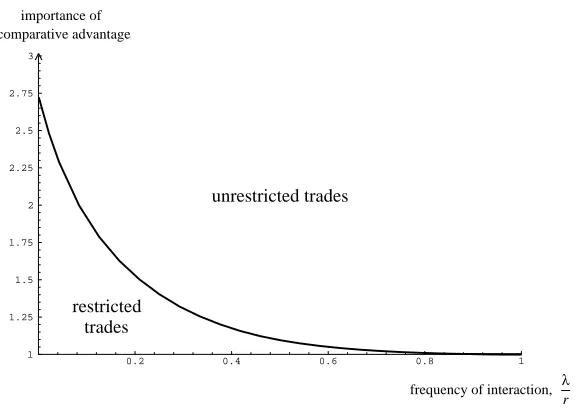
[image:24.612.164.455.360.569.2]The implications of this section are illustrated in Figure 7.
Figure 7: Optimal Regions for Restricted Networks
0.2 0.4 0.6 0.8 1
1 1.25 1.5 1.75 2 2.25 2.5 2.75 3 ^
unrestricted trades
restricted trades
frequency of interaction, λ
r
importance of comparative advantage
Here we illustrate situations in which it is efficient to restrict networks in terms of frequency
of interaction (λr) and the importance of comparative advantage (α). Below the curve drawn, it
is efficient for individuals to only trade with one trading partner. They will forego the benefits of
comparative advantage (i.e., trading with all three individuals), but can support more trade with
their single trade partner when they are more reliant on one another. Above the line, agents should
form more diverse links. Note that the line is downward sloped, which implies that as interactions
The formal model above is simply meant to emphasize the importance of dense trade for
reci-procity to operate. As a result, individuals may dedicate a large fraction of their trades to a single
agent, even though that agent may not be the most effective provider of that good. At a more
informal level, it also points to a difficulty which smaller firms may have in the network process.
Although these new smaller firms may be more efficient providers of goods in the usual cost sense,
trade partners may be hard to find as they see the importance of their existing networks, which
though sometimes inefficient, are at least trustworthy.
6
Liquidity Shocks and Prices
So far, we have largely looked at barter arrangements as if there was not a money market also
operating in tandem. This section, based on Prendergast and Stole (1999), begins to address
what we feel is an important but unexplored topic in the context of barter societies, namely, the
interaction between many currencies which simultaneously circulate, as occurs in Russia. It remains
very unclear how these currencies interact with one another; their effects are hardly neutral on each
other but exactly how the existence of rubles affects the use of pasta or social contacts remains
unclear. Central to current trading in Russia is the absence of liquidity that drives much of barter
trade. Our interest in this section specifically is in understanding the response of prices to a
liquidity shock. To describe the issue, consider the following trivial example. Suppose that before
the August 1998 shock everyone in Russia had £2 but that after the shock, liquidity dried up so
that everyone has£1. An immediate question that arises is why don’t prices adjust such that the
real quantity of money is unchanged. In other words, why aren’t prices simply cut in two?
Our answer to this relies on two building blocks.25 First, we assume that prices may not be set
competitively.26 To model non-competitive setting of prices, we consider the standard monopoly
25
As in the other sections of the paper, we do not provide much technical detail but instead offer an example which illustrates some of the relevant effects. This example is based on Prendergast and Stole (1999). The reader is referred there for more details.
26
setting where there is uncertainty about the valuation of a buyer for the seller’s good. We assume
that when a seller is offering his good to a buyer, the buyer values a single unit of the good at v,
wherev is uniformly distributed between 0 and 1. Only the buyer knows how much he values the
good. Assume further for simplicity that the quantity supplied is discrete, equal to either 0 or 1,
and that the cost of the good is zero. As a result, of these assumptions, it is always efficient (but not
necessarily most profitable) to supply the good. If there are no other constraints or opportunities,
it is simple to show that the monopoly seller would choose his price to be 12. In such a case, only
half the population (those with valuations above 12) would buy, but profits would be greater than
at any other price.
The additional assumption we make, however, is that there are liquidity shocks, where the
buyer may be liquidity constrained with not enough money to pay for the good. To fix this idea,
we assume that he has m units of currency with which he can buy the good. Then his “effective
willingness to pay” will be the minimum of his valuationvand his money stockm. This represents
a simple way to analyze the effects of liquidity.27 However, importantly, not everyone is affected
equally by the liquidity shock. Specifically, we assume that those who have low valuations are also
likely to have little money. Put in loose terms, poor people are less likely to buy and are also those
who are most affected by shocks to liquidity. Those in wealthier initial positions are more likely
buyers because (i) they are more willing to buy the good if they have money and (ii) are more likely
to have money even after the liquidity shock, perhaps because of their better positions in trading
networks, as described in Section 4.
One natural way to model this is through a correlation between valuations and money holdings.
We use a particularly simple form of correlation, where we assume that m = a+bv, a < 0 and
b > 1.28 In other words, a 1 unit increase in valuations increases money stocks by b. What this
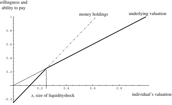
means can be most easily seen from Figure 8, where we have taken a simple example in which
b= 1.25 anda=−0.25.
27
Some readers may be uncomfortable with defining inherent valuations independently of money holdings. The simplest way to think of this is thatmrefers to a distinct composite good, where the marginal value of the seller’s good (relative to the composite) isv.
28
Figure 8: The Effect of Liquidity Shocks on Willingness to Pay
0.2 0.4 0.6 0.8
-0.2 0.2 0.4 0.6 0.8
1 money holdings underlying valuation
willingness and ability to pay
individual’s valuation z, size of liquidityshock
The dark shaded line represents the effective willingness to pay. For those who have high
valuations (above z in Figure 8), the underlying valuation of the buyer is less than his money
holdings. In other words, liquidity constraints are not important for that person, as he has enough
money to pay for the good. However, this is not true for all individuals who value the good at less
thanz. In that case, the agents do not have enough money to pay their valuation: instead all that
they can pay is their money holdings, m.29
Start by imagining that there are no opportunities for barter: this is not meant to reflect current
reality in Russia, but is simply a counterfactual against which we will consider a world with barter.
What we are most interested in is how prices are affected by the liquidity shock. Now remember
from Figure 8 that those who have valuations below z are liquidity constrained. Therefore, as z
gets bigger, the environment becomes more liquidity constrained. (This is equivalent to decreasing
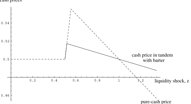
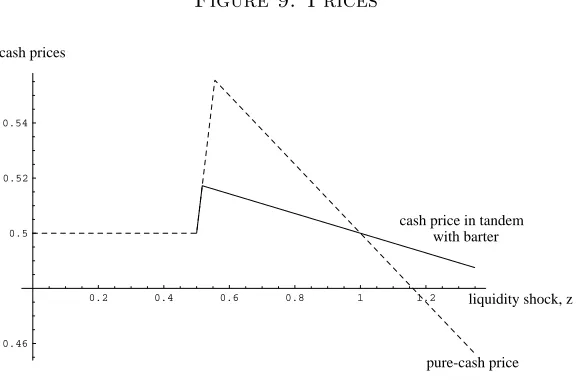
a with the technology above.) The hatched line in Figure 9 gives optimal prices which arise as a
function of the liquidity shock.
29
Figure 9: Prices
0.2 0.4 0.6 0.8 1 1.2
0.46 0.5 0.52 0.54 cash prices
pure-cash price cash price in tandem
with barter
liquidity shock, z
It is simplest to begin at the two extremes: (a) where zis low (less than 12), so few are liquidity
constrained, and (b) where z exceeds 1, so everyone is liquidity constrained. First, when few are
liquidity constrained, the price charged is 12, unchanged from the case where there is no liquidity
shock. This arises simply because the only people affected by the shock are those who would not
have bought anyway: hence the optimal price is unchanged. When the liquidity shock is large,
specifically when z > 1, everyone is affected by the shock. In this case, prices fall below the their
level when there is no liquidity shock. This reflects the imagined direct effect of an absence of
liquidity on prices: if people don’t have any money, you should not demand as much as when they
do.
However, the intermediate regions are also of interest, as they illustrate how liquidity shocks
cause sellers to increase prices over some range and then to reduce them. This arises for the
following reason. Consider a liquidity shock which causes some marginal buyers (those around 12)
to be liquidity constrained. One possibility is to reduce the price to pick these up: but this reduces
the revenues on those with higher valuations who would have bought anyway. An alternative is
to ignore these customers and choose a price at which only those who have high valuations (and
money holdings) will buy. For intermediate ranges of liquidity shocks, the latter effect always
dominates, so the optimal pricing strategy is to increase the price as customers initially become
liquidity constrained in the relevant demand region. In short, the liquidity shock decimates the
demand of the moderate purchasers, so it now is more profitable for the seller to focus attention
on the cash market’s high end purchasers.
But firms have another option which we have so far ignored: they can barter their goods through
repeated barter environment as we have done in the previous sections, we instead simply consider a
“reduced form” structure of barter where we note that there is some cost to trading through barter
rather than directly selling for cash. This could be the cost which must be paid to a middleman, as
in Section 4, or the inefficient production which arises when goods are not equally valued by both
parties, as in Section 3.1. Specifically, we assume that there is a “tax” on barter which reflects
this: where a unit of the buyer’s “commodity cash” (i.e., the goods which the buyer transfers to
the seller in exchange for satisfying the buyer’s demands) has value x to the seller (in terms of
the composite), but which costs tx to the buyer to generate. We assume thatt >1, reflecting the
standard inefficiencies of barter.
How does the opportunity for barter affect the cash market? Clearly, it now gives sellers the
opportunity to sell their goods not only for cash but also they can offer their goods for barter also.
This provides them with an additional outlet for their goods which increases their profitability,
but importantly also gives buyers an alternative option, where they can barter instead of buying
for cash. The solid line in Figure 9 plots optimal money prices when barter is also an option. In
this figure, we assume that t= 1.5.30 Our primary focus is on the difference between the hatched
line and the full line: in other words, how does the existence of barter exchange affect money
pricing? Again, consider the extremes. When the liquidity constraints are not important, there is
no difference in the price charged, for the reason that the barter market is never used.31 At the
other extreme, wherez >1, when liquidity constraints are extreme, prices when barter is an option
are still lower than when there is no liquidity problem. However, they are higher than when only
the cash market operated. In other words, the existence of the barter market mutes the incentive to
reduce prices with liquidity shocks. In this region, both currencies circulate simultaneously, where
those with high enough valuations (and money) use the cash market while those who do not will
use the barter market. Why is it that prices are higher when barter is an option? The reason is
that the benefits to a price reduction in a world without barter are that customers who would not
otherwise buy the product now will purchase it at the lower price. When barter is present, a price
reduction (holding the barter terms fixed) will only serve to convert bartering buyers into cash
buyers. While this is profitable to the seller, conversion is not as profitable as new sales. Hence,
the presence of bater mutes the incentive to reduce prices when liquidity shocks hit the system.
Thus multiple currencies interact in non-trivial ways.32
30
The more general importance of this assumption is that for the example we have computed it is the case that
t≥b. We have not yet analyzed the case where this condition does not hold. 31
One might imagine that those buyers without money would be offered the opportunity to barter in this region. However, this is not the case because there is the temptation that those who would otherwise pay with cash will now switch to barter. The cost of this transition is enough to cause the firm to offer no barter swaps.
32