Design of a Simulator for Enhanced Oil Recovery Process Using a Nigerian Reservoir as a Case Study

http://dx.doi.org/10.4236/aces.2014.44047

How to cite this paper: Oyedeko, K.F. and Susu, A.A. (2014) Design of a Simulator for Enhanced Oil Recovery Process Using a Nigerian Reservoir as a Case Study. Advances in Chemical Engineering and Science, 4, 430-453.

http://dx.doi.org/10.4236/aces.2014.44047

Design of a Simulator for Enhanced Oil

Recovery Process Using a Nigerian

Reservoir as a Case Study

Kamilu Folorunsho Oyedeko

1*

_{, Alfred Akpoveta Susu}

2

1_{Department of Chemical & Polymer Engineering, Lagos State University, Epe, Lagos, Nigeria} 2_{Department of Chemical Engineering, University of Lagos, Lagos, Nigeria}

Email: *_{kfkoyedeko@yahoo.com, alfredasusu222@hotmail.com} Received 21 July 2014; revised 18 August 2014; accepted 28 August 2014 Copyright © 2014 by authors and Scientific Research Publishing Inc.

This work is licensed under the Creative Commons Attribution International License (CC BY).

http://creativecommons.org/licenses/by/4.0/

Abstract

This study involves the applications of different numerical techniques in a more general way to the design of a simulator for an enhanced oil recovery process with surfactant assisted water flooding. The data from a hypothetical oil well and a Nigerian oil well were used for the validation of the simulator. The process is represented by a system of nonlinear partial differential equations: the continuity equation for the transport of the components and Darcy’s equation for the phase flow. The orthogonal collocation, finite difference and coherence theory techniques were used in solving the equations that characterized the multidimensional, multiphase and multicomponent flow problem. Matlab computer programs were used for the numerical solution of the model equ- ations. The predicted simulator, obtained from the resulting numerical exercise confers uncondi- tional stability and more insight into the physical reservoir description. The results of the ortho- gonal collocation solution were compared with those of finite difference and coherence solutions. The results indicate that the concentration of surfactants for orthogonal collocation show more features than the predictions of the coherence solution and the finite difference, offering more opportunities for further understanding of the physical nature of the complex problem. We have found out that the partition of the three components between the two-phases determines other physical property data and hence the oil recovery. The oil recovery for the Nigerian oil reservoir is higher than the recovery predicted for the hypothetical crude. The displacement mechanism for the multicomponent and multiphase system is stable in the Nigerian oil reservoir due to the mod- erate value of the oil/water viscosity instead of the hypothetical reservoir with high value of oil/water ratio.

Keywords

Enhanced oil Recovery, Simulator Design, Multidimensional, Multicomponent and Multiphase

System, Surfactant Assisted Flooding, Orthogonal Collocation, Finite Difference, Coherence Theory, Hypothetical Reservoir, Nigerian Reservoir

1. Introduction

The world economy today can be characterized as a crude oil economy. So far, there has not been a single ener-gy source that has broadly been integrated to replace crude oil in the provision of electricity (light and heat) and transportation (land, air and sea). It is very important to at least, maintain or indeed, increase the current produc-tion levels of crude oil. These objectives can be accomplished by further investing in exploraproduc-tion and producproduc-tion of new fields or optimizing production from existing fields. Bringing new fields online can be expensive, while recovery from existing fields by conventional methods (i.e. primary and secondary recovery) will not fully pro-vide the necessary relief for global oil demand.

On an average, only about a third of the original oil in place can be recovered by primary and secondary re-covery processes. The rest of the oil is trapped in reservoir pores due to surface and interfacial forces. This trapped oil can be recovered by reducing the capillary forces that prevent oil from flowing within the pores of reservoir rock and into the well bores. Due to high oil prices and declining production in many regions around the globe, the application of advance technologies called “Enhanced Oil Recovery” (EOR) has become very at-tractive for exploration and production of the trapped oil. This technology requires the injection of a fluid or fluids or materials into a reservoir to supplement the natural energy present in a reservoir, where the injected fluids interact with the reservoir rock/oil/brine system to create favourable conditions for maximum oil recovery. Surfactants are injected to decrease the interfacial tension between oil and water in order to mobilize the oil trapped after secondary recovery by water flooding.

In a surfactant flood, a multi-component multiphase system is involved. The theory of multi-component, mul-tiphase flow has been presented by several authors. The surfactant flooding is a form of chemical flooding and is represented by a system of nonlinear partial differential equations: the continuity equation for the transport of the components and Darcy’s equation for the phase flow. The system of equations is completed by the equations representing physical properties of the fluids and the rock. From a physico-chemical point of view, there are three components—water, petroleum and chemical. They are in fact, pseudo-components, since each one con-sists of several pure components. Petroleum is a complex mixture of many hydrocarbons. Water is actually brine, and contains dissolved salts. Finally, the chemical contains different kinds of surfactants. These components are distributed between two phases—the oleic phase and the aqueous phase. The chemical has an amphiphilic cha-racter. It makes the oleic phase at least partially miscible with water or the aqueous phase, partially miscible with petroleum.

Interfacial tension depends on the surfactant partition between the two phases. Residual phase saturation de-creases as interfacial tension dede-creases. Relative permeability parameters depend on residual phase saturations. In addition, phase viscosities are functions of the volume fraction of the components in each fluid phase. There-fore, the success or failure of surfactant flooding processes depends on phase behaviour. Phase behaviour influ-ences all other physical properties, and each of them, in turn influinflu-ences oil recovery.

The different mathematical techniques used here, orthogonal collocation method, finite difference and cohe-rence theory methods, are utilized for identification of particular physical behaviour. Besides, they may enable the understanding of the involved propagation phenomena in terms of cause and effects. More so, the techniques will in particular be utilized to predict what happens in EOR process and show how the complexity of the prob-lem can be reduced by intensive calculation.

in groundwater systems by adjusting the number of particles served to maintain an accurate material balance and save computational time. This front-tracking approach has been used in the present work to trace the movement of coherent waves, of both the diffuse and shock variety.

The concept of coherence was extended to general EOR processes [4] [5], including alkaline flooding [6], convectional surfactant flooding [7] the effects of cation-exchange on surfactant-polymer flooding [8] [9] and miscible gas injection processes such as CO2 flooding (Orr et al., 1995; Wang and Orr, 1997). Refinements to

the theory also allowed for equilibrium reaction to occur, such as precipitation-dissolution [10] [11] and micelle formation [12]. Helset and Lake [13] have used simple wave theory (essentially identical to coherence theory) to study the one dimensional, three phase secondary migration of hydrocarbons from a source rock into possible reservoirs. Most recently, the theory of coherence has been applied successfully to the analysis of the transport of volatile compounds in porous media in the presence of a trapped gas phase [14].

At the simple level, the results of simulation using the principle of coherence are analogous to the Buck-ley-Leverett theory for water flooding, the latter being evident in the work of Patton et al. [15] for polymer flooding, Fayers and Perrine [16] for dilute surfactant flooding, Claridge and Bondor [17] for carbonated water flooding and Larson [18] and Hirasaki [7] for miscible and immiscible surfactant flooding, respectively. Pope, et

al. [19] for isothermal, multiphase, multicomponent fluid Flow in permeable media. Hankins and Harwell [20].

Case studies for the feasibility of sweep improvement in surfactant-assisted water flooding. Other works on EOR researches include the work of Siggel, et al. [21] for a new class of viscoelastic surfactants for EOR, Xu and Lu [22] for microbially enhanced oil recovery at simulated reservoir conditions by use of engineered bacteria, Andrew Leach and Mason [23] for co-optimization of enhanced oil recovery and carbon sequestration, Harwell [24] for development of improved surfactants and EOR methods for small operators and many others.

So, in this work, we apply the different numerical techniques, orthogonal collocation, finite difference and coherence theory method, in solving the basic model transport equations characterizing the design of the simu-lator. As far as the authors are aware, this is the first time that the orthogonal collocation method is being ap-plied to simulator design. The approach is multidimensional and involves at least three independent variables with the introduction of the concept of partial coherence so that the various composition path spaces required for mapping the composition routes of the system are at most two dimensional.

2. Methodology

In this work, we considered solving multidimensional, multicomponent, multiphase flow problems associated with enhanced oil recovery process in petroleum engineering. The process of interest involves the injection of surfactant of different concentrations and pore volume to displace oil from the reservoir.

The methodology indicates the steps utilized in executing the project using the developed mathematical mod-els to describe the physics of reservoir depletion and fluid flow in which one of the main aims is the determina-tion of the areal distribudetermina-tion of fluids in the reservoir resulting from a flood. The system is for two or three di-mensions, two fluid phases (aqueous, oleic) and one adsorbent phase, four components (oil, water, surfactants 1 and 2).

The reservoir may be divided into discrete grid blocks which may each be characterized by having different reservoir properties. The flow of fluids from a block is governed by the principle of mass conservation coupled with Darcy’s law. The simultaneous flow of oil, gas, and water, in three dimensions and the effects of natural water influx, fluid compressibility, mass transfer between gas and liquid phases and the variation of such para-meters as porosity and permeability, as functions of pressure are then modelled.

The model is developed from the basic law of conservation of mass [25]. The developed partial differential equation is converted to ordinary differential equation using coherent, finite difference and orthogonal colloca-tion methods.

The finite difference method is a technique that converts partial differential equations into a system of linear equations. There are essentially three finite difference techniques. The explicit, finite difference method converts the partial differential equations into an algebraic equation which can be solved by stepping forward (forward difference), backward (backward difference) or centrally (central difference).

trun-cation error over the required for other methods.

The coherent theory method combines the forward finite difference method with Runge Kutta technique to solve partial differential equations.

The rock and fluid properties such as density, porosity, viscosity, oil and water etc, and other parameters are listed inTables 1-4. Table 1 is the Reservoir characteristics from the work by Hankins and Harwell [25].Table 2 is the Reservoir Characteristics used for the Simulation work by Oyedeko [26]. Parameter values used in Tro-gus adsorption model for verification runs is shown in Table 3while Table 4 is the Additional Reservoir Para-meters for the coherence work by Hankins and Harwell [25].

The model encompasses two fluid phases (aqueous and oleic), one adsorbent phase (rock), and four compo-nents (oil, water, surfactants 1 and 2). The oil is displaced by water flooding. In-situ interaction of surfactant slugs may occur, with consequent phase separation and local permeability reduction. The model accommodates two (or three) physical dimensions, and an arbitrary, nonisotropic description of absolute permeability variation and porosity.

[image:4.595.92.504.321.716.2]

For most of the simulated cases in the work of Harkins and Harwell [25], the reservoir consisted of a rectan-gular composite of horizontal oil bearing strata, sandwiched above and below by two impervious rocks. Oil is produced from the reservoir by means of water injection at one end and a production well at the other. Data for the hypothetical reservoir simulated in Hankins and Harwell [25] are given in Table 6and the model developed is given as:

Table 1. Reservoir characteristics from the work of Hankins and Harwell [25].

Parameter Value

Rock density 2.65 g/cm3

Porosity 0.2

Oil viscosity 5.0 cp

Water viscosity 1.0 cp

Injection pressure gradient (maintained constant) 1.5 psi/ft

Fluid densities 1.0 g/cm3

Width of injection face 50 ft

Width of central high permeability streak 10 ft

Length of reservoir 100 or 5000 ft

Residual oil saturation 0.2

Connate water saturation 0.1

First injected surfactant SDS

Second injected surfactant DPC

Henry’s law constant SDS DPC

2.71 × 10−4 l/g 8.30 × 10−5 l/g

CMC values SDS DPC

800 μmol/l 4000 μmoll/l

Injected concentration SDS DPC

10 CMC 10 CMC

Brine spacer (typical) ≈0.05 pore volumes

[image:5.595.96.502.104.555.2]

Table 2.Reservoir characteristics used for the simulation work by Oyedeko [26].

Parameter Value

Rock density 2.65 g/cm3

Porosity 0.2

Oil viscosity 0.40 cp

Water viscosity 0.30 cp

Injection pressure gradient (maintained constant) 1.5 psi/ft

Fluid densities 1.0 g/cm3

Width of injection face 50 ft

Width of central high permeability streak 10 ft

Length of reservoir 100 or 5000 ft

Residual oil saturation 0.2

Connate water saturation 0.2

First injected surfactant SDS

Second injected surfactant DPC

Henry’s law constant SDS DPC

2.71 × 10−4 l/g 8.30 × 10−5 l/g

CMC values SDS DPC

800 μmol/l 4000 μmoll/l

Injected concentration SDS DPC

10 CMC 10 CMC

Brine spacer (typical) ≈0.05 pore volumes

[image:5.595.99.498.505.720.2]

Slug volumes ≈ 0.10 pore volumes

Table 3. Parameter values used in Trogus adsorption model for verification runs.

Parameter Value

Pure component CMCs

3 1 1.0 mol m

C∗=

3 2 0.35 mol m

C∗=

Phase separation model parameter Θ = 1.8

Henry’s law constants for adsorption

,

i i i w

C =k C

(Ci w, = aqueous monomer concentration)

k1 = 0.21 × 10−3 m3/kg

k2 = 0.80 × 10−3 m3/kg

Henry’s law constant for oleic partitioning

, ,

i o i i w

C =q C

(Ci w, = aqueous monomer concentration)

q1 = 7.1

q2 = 1.3

Adsorbent properties ρs = 2.1 × 10

+3 _m3_/kg

[image:6.595.90.505.98.361.2]

Table 4. Additional reservoir parameters for the coherence work by Hankin and Harwell [25].

Model designation A B

Grid points in the horizontal direction (m + 1) 21 21

Grid points in the vertical direction (n + 1) 11 21

Coherent waves of water saturation 28 28

Initial number of points per coherent wave Water

Surfactant

41 81

41 81

Maximum number of points required per coherent wave ≈300 ≈300

Average time step size (days) Short reservoir (100 ft)

200 mD streak 1000 mD streak Long reservoir (5000 ft)

200 mD streak 1000 mD sreak

3.47 0.69

174.0 34.7

3.47 0.69

174.0 34.7

Typical number of time steps required to inject first pore volume Short reservoir

Long reservoir

33 75

33 75

(

)

(

)

, , ,

1 1, 2

i w i i w i w

w x w y w i

C C C C

S v f v f r i

t t x y

φ ∂ +ρ −φ ∂ +φ ∂ +φ ∂ = − =

∂ ∂ ∂ ∂ (1)

The term r_i represents the rate of loss of surfactant due to precipitation: for a one-to-one reaction stoichi-ometry, r₁=r₂. Since reaction occurs instantaneously at a sharp interface, this term may be ignored away from the singular region of the interface.

It is possible to approximate the adsorption isotherm of a pure surfactant on a mineral oxide by use of a sim-ple model. At low concentration the adsorption obeys Henry’s law, while above the critical micelle concentra-tion (CMC) the total adsorpconcentra-tion remains constant. The Trogus adsorpconcentra-tion model [12] [27] is used in this work.

2.1. Application of Coherence Theory to the Solution of Model Equations

The material balance equations, Equation (1) (in the absence of r_i), are first order, homogeneous, nonlinear hyperbolic equations. Their solution will be attempted by means of the theory of coherence. The results pre-sented here are general, and not restricted to assumptions regarding equilibrium relationships, fractional flow relationships, etc.

The concept of coherence identifies the state which a dynamic, multi-component system strives to attain. The state of “coherence” requires all dependent variables at any given point in space and time to have the same wave velocity, giving rise to “a coherent” wave with no relative shift in the profiles of the variables. It has been estab-lished mathematically by Helfferich [28] that an arbitrary starting variation of dependent variables, if embedded between sufficiently large regions of constant state, is resolved into coherent waves, which become separated by new regions of constant state.

Oleic Partitioning

The model developed and expressed in Equation (1) may be generalized by allowing surfactants to partition into the oleic phase. In general, Ci o, =Ci o,

(

C1, ,wC2,w

)

this leads to:

(

)

, , , , , , ,

1

i w i o i w i w i w i o i o

w o x w y w x o y o i

C C C C C C C

S S v f v f v f v f r

t t t x y x x

φ ∂ +φ ∂ + −φ ρ∂ +φ ∂ +φ ∂ +φ ∂ +φ ∂ = −

∂ ∂ ∂ ∂ ∂ ∂ ∂ (2)

Leading to the matrix equation:

(

)

(

)

(

21 1121

)

21 11

(

2212 1222

)

12 22 2,1,

0 w

w o ii w o o o

w

o o w o w o

dC

S S p m f f p S p m f p

dC

S p m f p S S p m f f p

λ λ

λ λ

 + + − − + −   

× =

 _{+ − + + − −}   

 

where

, ,

,

, 1 , 1

i o

i j o w o w

j w C

p f f S S

C

∂

= = − = −

∂

2.2. Application of Finite Difference to the Solution of Model Equations

First-order, finite-difference expressions for the spatial derivatives were substituted into the hyperbolic chroma-tographic transport equations (Equation (1)), yielding 2× m coupled ordinary differential equations which may then be integrated simultaneously (also known as the “numerical method of lines”).

(

)

(

)

(

)

2

, , , , 1

1

, ,

, 0

i w i w i w h i w h

w ij w h

j

C C C C

s m f τ ε τ ε τ ε

τ τ ε

−

=

 

∂ ∂ _ − _

+ + × =

∂

∑

∂ _ ∆ _ (4)

where i=1, 2 and

h

=

1, 2,



,

m

.

Equation (4) is the finite-difference form of Equation (1) written for one spatial dimension

ε

, where m_ij are the adsorption coefficients,

τ

is dimensionless time (injected volume/pore volume), and

ε

is dimension-less distance (pore volumes travelled). In two dimensions, the finite-difference terms are multiplied by dimen-sionless velocities. The distortion of the solution in the

τ

direction may be neglected by using a 4th order Runge-Kutta method and a sufficiently small time step.

The above equation is now transformed to the original form of Equation (1) using the already defined va-riables below

, ,

i w i w

C′ =φC (5)

(

1

)

i i

C′=

ρ

−

φ

C′ (6)

, , i i j j w C m C ′ ∂ = ′

∂ (7)

Again, recall that differentiation of a function of another function (chain rule) is of the form

y y u

x u x

∂ ₌ ∂ _×∂

∂ ∂ ∂ (8)

Applying the chain rule above, Equation (4) becomes

(

)

(

)

(

)

, 1, 2, , , 1

1, 2,

, ,

, 0

i w i w i w i w h i w h

w w h

w w

C C C C C C C

S f

C C

τ ε τ ε

τ ε

τ τ τ ε

−

′  ′   ′   ′ ′ 

∂ ₊ ∂ ′ _⋅∂ ₊ ∂ ′ _⋅∂ _{+ ×} − ₌

     

 _′   _′ 

∂ _∂ ∂ _{ }∂ ∂ _{ } ∆ _ (9)

Eliminating the primes (') and bars (−) and introducing m_{i j,} terms yield

(

)

1, 2, 1,

11 12 0

w w w

w w

C C C

S m m f

τ

τ

ε

∂ ∂ ∂

+ + + =

∂ ∂ ∂ (10)

(

)

2, 1, 2,

22 21 0

w w w

w w

C C C

S m m f

τ

τ

ε

∂ ∂ ∂

+ + + =

∂ ∂ ∂ (11)

Applying the method of lines, a partial transformation to a difference equation, to the equations above yield:

(

)

1, 2, 1, (, ) 1, (, 1)

11 12 0

h h w w w w w w C C C C

S m m f τ ε τ ε

τ τ ε

− −

∂ ∂

+ + + =

∂ ∂ ∆ (12)

(

)

2, 1, 2, (, ) 2, (, 1)

22 21 0

h h w w w w w w C C C C

S m m f τ ε τ ε

τ τ ε

− −

∂ ∂

+ + + =

∂ ∂ ∆ (13)

This can also be written as follows:

(

)

( ) ( )

( ) ( )

, ,

, , 1

1, 2,

11 12 1, 1, 0

h h

h h

w w

w

w w w

C C _f

S m τ ε m τ ε C C

τ ε τ ε

τ τ ε −

∂ ∂

 

+ + + _ − _=

 

(

)

( ) ( )

( ) ( )

, ,

, , 1

2, 1,

22 21 2, 2, 0

h h

h h

w w

w

w w w

C C _f

S m τ ε m τ ε C C

τ ε τ ε

τ τ ε −

∂ ∂

 

+ + + _ − _=

∂ ∂ ∆ (15)

Since we have a set of simultaneous ODE’s, we will attempt to solve the equations:

(

)

( ) ( )

( ) ( )

, ,

, , 1

1, 2,

11 12 1, 1, 0

h h

h h

w w

w

w w w

C C _f

S m τ ε m τ ε C C

τ ε τ ε

τ τ ε −

∂ ∂

 

+ + + _ − _=

 

∂ ∂ ∆ (16)

(

)

( ) ( )

( ) ( )

, ,

, , 1

2, 1,

22 21 2, 2, 0

h h

h h

w w

w

w w w

C C _f

S m τ ε m τ ε C C

τ ε τ ε

τ τ ε −

∂ ∂

 

+ + + _ − _=

∂ ∂ ∆ (17)

where

1 1 2 2

11 12 21 22

1, 2, 1, 2,

, , ,

w w w w

C C C C

m m m m

C C C C

∂ ∂ ∂ ∂

= = = =

∂ ∂ ∂ ∂ (18)

Substituting for these terms in Equations (16) and (17) yield

( ) ( )

( ) ( )

, ,

, , 1

2, 1, 2 2 2, 1, 2, 1, 0 h h h h w w w

w w w

w w

C C _f

C C

S C C

C C

τ ε τ ε

τ ε τ ε

τ τ ε −

∂ ∂

 ₊ ∂  ₊ ∂ _{+  − =}

  _{ }

 ∂  ∂ ∂ ∂ ∆  

  (19)

And

( ) ( )

( ) ( )

, ,

, , 1

2, 1, 2 2 2, 2, 2, 1, 0 h h h h w w w

w w w

w w

C C _f

C C

S C C

C C

τ ε τ ε

τ ε τ ε

τ τ ε −

∂ ∂

 ₊ ∂  ₊ ∂ _{+  − =}

  _{ }

 ∂  ∂ ∂ ∂ ∆  

  (20)

These on simplification yield

( ) ( ) ( ) ( ) ( ) ( ) ( ) ( ) ( ) ( ) ( ) , , ,

, , 1

,

, , 1

,

, , 1

1, 1, 2,

1 1 1, 1, 1, 2, 1, 1 1 1, 1, 1, 1 1, 1,

. . 0

0

2 0

simi

h h h

h h

h

h h

h

h h

w w w

w

w w w

w w

w

w

w w w

w

w

w w w

C _C C _C C _f

S C C

C C

C _{C C f}

S C C

C _{C f}

S C C

τ ε τ ε τ ε

τ ε τ ε

τ ε

τ ε τ ε

τ ε

τ ε τ ε

τ τ τ ε

τ τ τ ε

τ τ ε

− − − ∂ _∂ ∂ _∂ ∂   + + + _ − _=   ∂ ∂ ∂ ∂ ∂ ∆ ∂ _{∂ ∂}   + + + _ − _=   ∂ ∂ ∂ ∆ ∂ _∂   + + _ − _=   ∂ ∂ ∆ ( ) ( ) ( ) ,

, , 1

2, 2 2, 2, larly 2 0 h h h w w

w w w

C _{C f}

S τ ε C C

τ ε τ ε

τ τ ε −

∂ _∂   + + _ − _=   ∂ ∂ ∆ (21)

From the Trogus model,

1 1 1, 2 2 2,

w

w

C k C

C k C

=

= (22)

A final substitution results in the equation below

( )

(

)

( ) ( ) ( ) ( ) ( )

(

)

_{( ) ( )} ( )

(

)

( ) ,

, , 1

,

, , 1

, , 1

,

,

1, _{1 1,}

1, 1,

1,

1,

1 1, 1,

1,

1 1, 1,

2, _{2 2,}

2, 2 2 0 2 0 2 0 and 2 h h h h h h h h h h w _w w

w w w

w

w w

w w w

w w

w w w

w _w

w

w w

C _{k C f}

S C C

C _{C f}

S k C C

C f

S k C C

C _{k C f}

S C C

τ ε

τ ε τ ε

τ ε

τ ε τ ε

τ ε τ ε

τ ε

τ ε

τ τ ε

τ τ ε

τ ε

τ τ ε

− − − ∂ _∂   + + _ − _= ∂ ∂ ∆ ∂ _∂   + + _ − _= ∂ ∂ ∆ ∂ _{ } + + _ − _= ∂ ∆ ∂ _∂ + + − ∂ ∂ ∆ ( )

(

)

_{( ) ( )} , 1

, , 1

,

2,

2 2, 2,

0 2 0 h h h w w w

w w w

C f

S k C C

τ ε

τ ε τ ε

2.3. Application of Orthogonal Collocation to the Solution of Model Equations

Equation (9) can be written as

(

)

(

)

(

)

, , , , , 1

2 , 0

i w i i w h i w h

w w h

C C C C

S f τ ε τ ε τ ε

τ τ ε

−

′  ′ ′ 

∂ ₊ ∂ ′_{+ ×} − ₌

 

∂ ∂ _ ∆ _ (24)

(

)

(

)

(

)

(

)

, 1 , , , , 1

2 i , 0

i w i w h i w h

w w h

C

C C C

S f

ρ φ

φ φ τ ε φ τ ε

τ ε

τ τ ε

−   ∂ −         ∂_{     } −_{  } + + ×_{ }=

∂ ∂ _ ∆ _ (25)

(

)

(

)

(

)

(

)

, , , , , 1

2 1 , 0

i w i i w h i w h

w w h

C C C C

S f τ ε τ ε

φ ρ φ φ τ ε

τ τ ε

−

 

∂ _{+ −} ∂ _{+ ×} − ₌

 

∂ ∂ _ ∆ _ (26)

Now, from the Trogus model,

, i i i w

C =

κ

C (27)

(

)

(

,

)

(

)

(

)

(

)

, , , , , 1

2 1 i i w , 0

i w i w h i w h

w w h

C

C C C

S

κ

f

τ ε

τ ε

φ

ρ

φ

φ

τ ε

τ

τ

ε

−

∂  

∂ _ − _

+ − + ×_{ }=

∂ ∂ _ ∆ _ (28)

(

)

(

)

(

)

(

)

, , , , , , 1

2 1 , 0

i w i w i w h i w h

w i w h

C C C C

S f τ ε τ ε

φ κ ρ φ φ τ ε

τ τ ε

−

 

∂ _{+ −} ∂ _{+ ×} − ₌

 

∂ ∂ _ ∆ _ (29)

(

)

(

)

, , ,

2 1 , 0

i w i w i w

w i w h

C C C

S f

φ

κ ρ

φ

φ

τ ε

τ

τ

ε

∂ ∂ ∂

+ − + =

∂ ∂ ∂ (30)

(

)

,

(

)

,

2 1 i w , i w 0

w i w h

C C

S f

φ

κ ρ

φ

φ

τ ε

τ

ε

∂ ∂

+ − + =

 

 _{ ∂ ∂} (31)

Let

(

)

2 1 w i w R S B f

φ κ ρ φ

φ

=_ + − _

=

The above equations now become:

0

C C

R B

τ ε

∂ ₊ ∂ ₌

∂ ∂ (32)

where C is a function of both ε (dimensionless distance) and τ (dimensionless time). Using the method of orthogonal collocation, let C be approximated by the expression

( )

1

( ) ( )

1

,

N

I J I

I

C

τ ε

C

τ

X

ε

+

=

=

∑

(33)

Equation (33) can now be expressed as follows:

( ) ( )

1

1

0

N

I J I I

C

R B C

τ

X

ε

τ

ε

+

=

∂ ₊ ∂ ₌

∂ ∂

∑

(34)

( ) ( )

1

1

0

N

I J I I

C

R B C

τ

X

ε

τ

ε

+

=

∂ ₊ ∂ _{ =}

 

∂

∑

∂ (35)

( )

( )

1

1

0

N

J I I I

C

R B X

ε

C

τ

τ

ε

+

=

∂ ₊ ∂ _{ ⋅ =}

 

∂

∑

∂ (36)

( )

JI J I

a X ε

ε ∂ =

1 1 0 N J JI I I C

R B a C

τ

+

=

∂ _{+ =}

∂

∑

(38)

1 1 0 N J JI I I C B a C R

τ

+ = ∂ + =

∂

∑

(39)

1 1 N J JI I I C B a C R

τ

+ = ∂ = −

∂

∑

(40)

For I=1, 2, 3, 4,,N+1 Therefore,

[

1 1 2 2 3 3 4 4 1 1

]

J

J J J J JN N

C B

a C a C a C a C a C

R

τ + +

∂ _{= − + + + + +}

∂  (41)

Again J=1, 2, 3, 4,,N+1

Therefore the following system of ODE’s can be generated

[

]

[

]

[

]

[

]

1

11 1 12 2 13 3 14 4 1 1 1

2

21 1 22 2 23 3 24 4 2 1 1

3

31 1 32 2 33 3 34 4 3 1 1

4

41 1 42 2 43 3 44 4 4 1 1

1

11 1 1

N N N N N N N N N N N C B

a C a C a C a C a C

R

C B

a C a C a C a C a C

R

C B

a C a C a C a C a C

R

C B

a C a C a C a C a C

R

C B

a C a

R τ τ τ τ τ + + + + + + + + + + + ∂ = − + + + + + ∂ ∂ = − + + + + + ∂ ∂ = − + + + + + ∂ ∂ = − + + + + + ∂ ∂ = − + ∂     

[

2C2+aN+13C3+aN+14C4+ + aN+1N+1CN+1

]

(42)

In matrix form, we have the following expression.

( )

( )

( )

( )

( )

1

2 11 12 13 14 1 1 1

21 22 23 24 2 1 2

3

31 3 1 3

41 4 1 4

4

11 12 1 1 1

1

N

N

N

N

N N N N N

N C

C a a a a a C

a a a a a C

C

a a C

B

R a a C

C

a a a C

C τ τ τ _τ τ τ τ τ τ τ + + + + + + + + + + ∂    _∂     ∂      _∂           ∂      _∂ _{= −}          _∂  _{  }  _∂                ∂   _∂                 (43)

Similarly, the following expression defines aJI[29] [30]

( )

_{( )}

( )

_{( )}

( )

_{( )}

( )

_{( )}

2 1 1 1 1 1 1 1 1 for 2 1 for N I N I JI N I

I J N J

P J I P a P I J P

ε

ε

ε

ε

ε

ε

( ) (

)

( )

( )

_{( ) (}

₎

( )

_{( )}

_{( )}

( )

_{( ) (}

₎

( )

_{( )}

( )

_{( )}

( )

_{( )}

_{( )}

( )

1 1 1 1 1

2 2 1

1 1

1 (2)

0 0

0

; 1, 2, 3, , 1

( 2

0

1

J J J

J J J J

J J J J

P P J N

P P P

P P P

P P

P

ε ε ε ε

ε ε ε ε ε

ε ε ε ε ε

ε ε ε − − − − − = − = + = − + = − + = = =  (45)

Recall that the elements of the matrix can be generated from the following Lagrange polynomial

( )

( )

_{( )}

( )

_{( )}

( )

_{( )}

( )

( )

2 1 1 1 1 1 1 1 1 2 d d ₁ N i N i j i ij N i

i j N j

P x

j i

P x

l x

a

x P x

i j

x x P x

+ + + +  =   = _{= }  _≠  −  (46)

For i = j, the elements here refer to the leading diagonal of the matrix to be generated. For i≠ j, the elements here refer to all other elements of the matrix.

Also, the following recurrence relations are defined below

( )

( )

(

)

( )

( )

_{( )}

(

)

( )

_{( )}

_{( )}

( )

_{( )}

(

)

( )

_{( )}

( )

_{( )}

1 1 1 1 1

2 2 1

1 1

1

2 o

j j j

j j j j

j j j j

p x

P x x x P x

P x x x P x P x

P x x x P x P x

− − − − − = = − = − + = − + (47)

For

j

=

2,3, 4,



,

N

+

1.

The following substitutions and manipulations will now be made to redefine Equation (46). Substituting the recurrence relations into Equation (46) yields

(

)

( )

_{( )}

_{( )}

(

)

( )

_{( )}

_{( )}

(

)

( )

_{( )}

_{( )}

(

)

( )

( )

( )

2 (1) 1 1 1 1 1 1 1 1 1 1 1 2 1 2 1

i j j i j i

i j j i j i

ij

i j j i j i

i j j j j j j j

x x P x P x

j i

x x P x P x

a

x x P x P x

i j

x x x x P x P x

− − − − − − − −   − +     =   − +     =   − +     ≠  −  − +   _{ }  (48)

Now, some terms will be cancelled out. Since j = i, (xi− xj) = 0,

And (xj− xj) = 0

( )

_{( )}

( )

(

)

( )

_{( )}

_{( )}

( )

1 1 1 1 1 1 1 2 1 2 1 j i j i ij

i j j i j i

i j j j

P x

j i

P x

a

x x P x P x

i j

x x P x

− − − − −       =  _ _  =   − +     ≠  −    _{ }  (49)

The above becomes

( )

_{( )}

( )

(

)

( )

_{( )}

(

) ( )

( )

( )

1 1 1 1 1 1 1 1 1 j i j i ij

i j j i j i

i j

i j j j j j

P x

j i

P x

a

x x P x P x

i j

x x

x x P x P x

This becomes ( )

_{( )}

( )

( )

_{( )}

( )

( )

( )

1 1 1 1 1 1 1 1 1 j i j i ij

j i j i

i j

j j j j

P x

j i

P x

a

P x P x

i j

x x

P x P x

− − − − − −     = _ _  =       + ≠  ₋    _{ }  (51)

Rewriting the above in terms of epsilon, (ε)

( )

_{( )}

( )

( )

_{( )}

( )

( )

( )

1 1 1 1 1 1 1 1 1 j i j i ij

j i j i

i j

j j j j

P j i P a P P i j P P ε ε ε ε ε ε ε ε − − − − − −     = _ _  =       + ≠  ₋    _{ }  (52)

The matrix now looks like this

( )

_{( )}

( )

1 0 1 11 0 1 P a P

ε

ε

= ( )

_{( )}

( )

( )

( )

1

1 1 1 1

12

1 2 1 2 1 2 1 P P a P P

ε

ε

ε ε

ε

ε

= + − ( )

_{( )}

( )

( )

( )

1

2 1 2 1

13

1 2 2 3 2 3 1 P P a P P

ε

ε

ε ε

ε

ε

= + − ( )

_{( )}

( )

( )

( )

1

0 2 0 2

21

2 1 0 1 0 1 1 P P a P P

ε

ε

ε

ε

ε

ε

= + − ( )

_{( )}

( )

1 1 2 22 1 1 P a P

ε

ε

= ( )

_{( )}

( )

( )

( )

1

2 2 2 2

23

2 3 2 3 2 3 1 P P a P P

ε

ε

ε

ε

ε

ε

= + − ( )

_{( )}

( )

( )

( )

1

0 3 0 3

31

3 1 0 1 0 1 1 P P a P P

ε

ε

ε ε

ε

ε

= + − ( )

_{( )}

( )

( )

( )

1

1 3 1 3

32

3 2 1 2 1 2 1 P P a P P

ε

ε

ε

ε

ε

ε

= + − ( )

_{( )}

( )

1 2 3 32 2 3 P a P

ε

ε

= (53)

The recurrence relations below will again be used to evaluate the terms of the matrix

( )

( )

(

)

( )

( )

_{( )}

(

)

( )

_{( )}

_{( )}

( )

_{( )}

1 1 1 1 1 1 0 1 0 o

j j j

j j j j

p

P P

P P P

P ε

ε ε ε ε

ε ε ε ε ε

Let ε assume the range ε = [0:0.01:0.09] where

1 0

ε = (55)

2 0.01

ε = (56)

3 0.02

ε = (57)

3. Results

The reservoir response, as predicted by the simulation on the basis of the theory of coherence, is compared with the numerical predictions obtained using traditional finite difference method and orthogonal collocation. For the case studies, data from a hypothetical well and an existing Nigerian well data were used for the validation of the simulation design. The main objective of these case studies has been to demonstrate that the mathematical tech-niques of orthogonal collocation, finite difference and coherent theory in the context of simulator design can be used to obtain wave behaviour in a reservoir. A gradually increasing level of complexity is introduced, repre- senting a range of systems from aqueous phase flow, to surfactant chromatography in two phase flow and to surfactant chromatography in two dimensional porous medium. The initial and injected surfactant compositions corresponding to Cases 1, 2 and 3 are shown in Table 5. The rock and fluid properties are listed in Tables 1-4. These properties are assumed uniform for convenience.

The two fluid phases consisted of a water phase and an oil phase, which, for convenience are considered in-compressible. The density of oil, the viscosity of oil, the salinity of water, and the formation volume factor of oil and water are listed in Table 2. All cases mentioned above were run by using anionic sodium dodecyl sulfate (SDS) and cationic dodecyl pyridinium chloride (DPC) as surfactants.

The system of equations is complete with the equations representing physical properties of the fluids and the rock. Physical properties described here are: 1) phase behaviour; 2) interfacial tension between fluid phases; 3) residual phase saturations; 4) relative permeabilities; 5) rock wettabiliy; 6) phase viscosities; 7) capillary pres-sure; 8) adsorption and 9) dispersion. From a physico-chemical point of view, there are three components—wa- ter, petroleum and chemical. They are in fact, pseudo-components, since each one consists of several pure com-ponents. Petroleum is a complex mixture of many hydrocarbons. Water is actually brine and contains dissolved salts. Finally, the chemical contains different kinds of surfactants.

These three pseudo-components are distributed between two phases—the oleic phase and the aqueous phase. The chemical has an amphiphilic character. It makes the oleic phase at least partially miscible with water or the aqueous phase partially miscible with petroleum.

Interfacial tension depends on the phase behaviour as the surfactant partitions between the two phases. Re-sidual phase saturation decreases as interfacial tension decreases. Relative permeability parameters depend on residual phase saturations. Phase viscosities are functions of the volume fraction of the components in each fluid phase. Therefore, the success or failure of surfactant flooding processes depends on phase behaviour. Also, phase behaviour influences all the other physical properties, and each of them, in turn influences oil recovery.

[image:13.595.92.505.636.719.2]

For a two-phase flow of water and oil, where no surfactant partitions into the oleic phase, the same scenario is obtained as the one dimensional injection for Cases 1 and 2. The bed has an initial water saturation of 0.3, and is flooded with an aqueous surfactant solution. The numerical profiles agree with the coherent wave profiles. The effect of the two-phase flow is to elongate the waves, leading to a larger region of constant state and earlier breakthrough of the fast wave.

Table 5.Conditions for case studies of surfactant chromatography Hankins and Harwell [25].

Case Injected composition: CC1 (mol/m3 _bed)

Injected composition: CC2 (mol/m3 _bed)

Initial composition: C1 (mol/m3 _bed)

Initial composition: C2 (mol/m3 _bed)

1 0.17 0.013 0.21 0.181

2 0.042 0.115 0 0

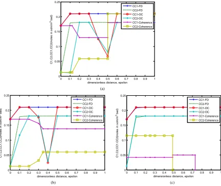
Figure 1(a) is the result obtained for solving Equation (4) using the three methods finite difference, orthogonal collocation, coherent theory. The graph is for the composition profile for one dimensional two-phase chromato-graphy initially equilibrated with a composition C1 = 0.21, C2 = 0.181 and is then injected with a composition C1

= 0.17, C2 = 0.013 (Riemann type problem Case 1, (refer to Table 5)). In Figure 1(a), the profile C1 of finite

difference shows a steady rise from C1 = 0.17 to C1 = 0.21 and then remain constant at this concentration. The

profile C1 of the orthogonal collocation increases steadily from C1 = 0.17 to C1 = 0.21 at distance 0.1 epsilon

maintaining a constant state to distance 0.3 epsilon. After this, it started declining from C1 = 0.21 to C1 = 0.07 at

distance 0.5 epsilon before rising back to attain a constant state with the finite difference. The profile C1 of the

coherent theory on the other hand started with a constant state, then declined before it reaches a constant state and then rises again to attain another constant state with the other profiles. Similarly, the profile C2 of finite

dif-ference increased steadily from C2 = 0.017 to a constant state of C2 = 0.18. The orthogonal collocation for C2

starts at C2 = 0.01 for a short constant state and then rises steadily to C2 = 0.18 to attain another short constant

state from 0.2 to 0.3 epsilon. From here it depressed to C2 = 0.07 before rising back to C2 = 0.18 and then attain

a constant state with finite difference. The profile C2 of coherent theory starts with a short constant state, then in-

creases readily to C2 = 0.05 for another constant state from where it rises up to the final region of constant state

with the other profiles.

(a)

[image:14.595.97.530.283.646.2]

(b) (c)

Figure 1. (a) Case 1. C1, C2vs epsilon at τ = 0.5. Bed composition profile for one-dimensional two-phase chromatography;

Case 1, at one-half pore volume injected. The plots are for three methods: Orthogonal collocation (OC), finite difference

(FD) and coherent theory (CT); (b) Case 1 C1, C2 vs epsilon at τ = 1.0. Bed composition profile for one-dimensional

two-phase chromatography; Case 1, at one pore volume injected. The plots are for three methods: Orthogonal collocation

(OC), finite difference (FD) and coherent theory (CT). (c) Case 1 C1, C2 vs epsilon at τ = 2.0. Bed composition profile for

one-dimensional two-phase chromatography; Case 1, at two pore volumes injected. The plots are for three methods:

Or-thogonal collocation (OC), finite difference (FD) and coherent theory (CT).

0 0.1 0.2 0.3 0.4 0.5 0.6 0.7 0.8 0.9 1

0 0.05 0.1 0.15 0.2 0.25

dimensionless distance, epsilon

C

1,

C

2,

C

C

1,

C

C

2(

m

ol

es

i

n s

ol

n/

m

3 bed)

CC1-FD CC2-FD CC1-OC CC2-OC CC1-Coherence CC2-Coherence

0 0.1 0.2 0.3 0.4 0.5 0.6 0.7 0.8 0.9 1

0 0.05 0.1 0.15 0.2 0.25

dimensionless distance, epsilon

C

1,

C

2,

C

C

1,

C

C

2(

m

ol

es

i

n s

ol

n/

m

3 bed)

CC1-FD CC2-FD CC1-OC CC2-OC CC1-Coherence CC2-Coherence

0 0.1 0.2 0.3 0.4 0.5 0.6 0.7 0.8 0.9 1

0 0.05 0.1 0.15 0.2 0.25

dimensionless distance, epsilon

C

1,

C

2,

C

C

1.

C

C

2(

m

ol

es

i

n s

ol

n/

m

3 bed)

Figure 1(b) shows the result obtained for solving Equation (4) by using orthogonal collocation and finite dif-ference as the numerical technique. The graph is for the bed composition profile for one dimensional two-phase chromatography for Case 1 at one pore volume injected. In this case also, the adsorbing porous medium is in-itially equibrated with a composition C1 = 0.21, C2 = 0.181 (concentrations normalized as moles in solution per

m3 of bed) and is then injected with a composition C1 = 0.17, C2 = 0.013 (Riemann-type problem: Case 1 (refer

to Table 5). The profile C1 for finite difference indicates a rise in concentration from C1 = 0.17 to 0.21 after

which the concentration maintained a constant state. The profile of C1 for the orthogonal collocation also rise

from C1 = 0.17 to C1 = 0.21 but falls to 0.03 epsilon at distance 0.4 epsilon and then increased thereafter to

con-stant state as maintained in the C1 profile for finite difference. The profile C1 of coherent theory started with a

constant concentration and then decreased gradually to attain another region of constant state. The profile C2 of

finite difference increased steadily from C2 = 0.02 to attain constant state at 0.18 epsilon. Also the profile of C2

of the orthogonal collocation increases gradually from C2 = 0.02 to C1 = 0.18 at distance 0.2 for a short constant

state and then decline to a low value of C2 = 0.02 at distance 0.4 epsilon before rising back to reach a constant

state with the finite difference profile. The profile C2 of coherent theory started with a constant state and

gradu-ally rises to a constant state

The bed composition profile for one dimensional two-phase chromatography for Case 1 at two pore volume injected is shown in Figure 1(c). This is the result obtained for solving Equation (4) by using these three tech-niques; finite difference, orthogonal collocation and coherent theory. The adsorbing porous medium is initially equibrated with a composition C1 = 0.21, C2 = 0.181 (concentrations normalized as moles in solution per m3 of

bed) and is then injected with a composition C1 = 0.17, C2 = 0.013 (Riemann-type problem: Case 1 (refer to

Ta-ble 5)). The profile C1 of finite difference and the profile C1 of orthogonal collocation indicate that there is

steady increase from C1 = 0.17 to C1 = 0.21 at distance 0.1 epsilon and then attained a constant state for both

profiles. However, the profile C1 of coherent theory shows a constant state of concentration at C1 = 0.04 before

having a self sharpening shock at C1 = 0.05, and eigenvalue λ = 0.499. It then continues at this constant state and

then decreased to zero at distance 0.73. Similarly, the profile C2 of finite difference shows a steady rise from C2

= 0.02 to C2 = 0.18 and then maintained a constant state. Also, the profile C2 for orthogonal collocation, follows

the same pattern, which indicates an increase from C2 = 0.02 to C2 = 0.18 and then attained a constant state. The

orthogonal collocation profiles match the finite difference profiles. However, the profile C2 of coherent theory

shows a constant state of concentration but has no self sharpening at C2 = 0.00 in this case before its termination

at distance 0.499 epsilon.

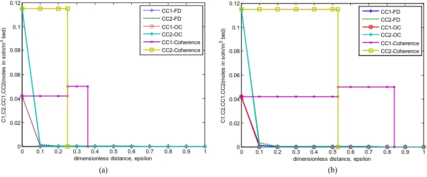
Figure 2(a)shows the bed concentration profiles for one dimensional two-phase chromatography for Case 2 at one pore volume injected in the porous medium initially devoid of surfactant and then injected with a mixture C1

(a) (b)

Figure 2. (a) Case 2, C1, C2 vs epsilon at τ = 1.0. Bed composition profile for one-dimensional two-phase

chromatogra-phy; Case 2, at one pore volume injected. The plots are for three methods: Orthogonal collocation (OC), finite difference

(FD) and coherent theory (CT); (b) Case 2. C1, C2 vs epsilon at τ = 2.0. Bed composition profile for one-dimensional

two-phase chromatography; Case 2, at two pore volumes injected. The plots are for three methods: Orthogonal colloca-tion (OC), finite difference (FD) and coherent theory (CT).

0 0.1 0.2 0.3 0.4 0.5 0.6 0.7 0.8 0.9 1

0 0.02 0.04 0.06 0.08 0.1 0.12

dimensionless distance, epsilon

C

1,

C

2,

C

C

1,

C

C

2(

m

ol

es

i

n s

ol

n/

m

3 bed)

CC1-FD CC2-FD CC1-OC CC2-OC CC1-Coherence CC2-Coherence

0 0.1 0.2 0.3 0.4 0.5 0.6 0.7 0.8 0.9 1

0 0.02 0.04 0.06 0.08 0.1 0.12

dimensionless distance, epsilon

C

1,

C

2,

C

C

1,

C

C

2(

m

ol

es

i

n s

ol

n/

m

3 bed)

[image:15.595.96.530.484.664.2]

= 0.042, C2 = 0.115 (Riemann-type problem, Case 2 (refer to Table 5), with the numerical result obtained for

solving Equation (4) by using three different techniques; orthogonal collocation, finite difference and coherent theory. The profile C1 of finite difference shows steady decline from C1 = 0.04 to a constant state, the same as

for orthogonal collocation. However, the profile C1 of coherent theory shows a constant state of concentration at

C1 = 0.04 before having a self sharpening shock at C1 = 0.048 and eigenvalue λ = 0.26. It then continues with a

constant state and decreased to zero at distance 0.37. The profile C2 of finite difference decreased steadily from

C2 = 0.119 to C2 = 0.001 and then to a constant state as for C1; a. similar behaviour was observed for orthogonal

collocation. Again, the profile C2 was different for coherent theory where a constant state was initially observed

with no self sharpening at C2 = 0.00.

The bed composition profile for one dimensional two-phase chromatography for Case 2 at two pore volume injected is shown in Figure 2(b). This is the result obtained for solving Equation (4) by using the three tech-niques; finite difference, orthogonal collocation and coherent theory. The profile of C1 for finite difference

shows steady decline from C1 = 0.04 to a constant state; similar behaviour was observed for orthogonal

colloca-tion. A difference was again observed for the profile C1 of coherent theory where the profile shows a constant

state of concentration at C1 = 0.04 before having a self sharpening shock of C1 = 0.046, and eigenvalue λ = 0.53.

It then continues with a constant state and decreased to zero at distance 0.84 epsilon. The profile C2 of finite

difference decreased steadily from C2 = 0.119 to C2 = 0.001 and then to a constant state as for C1; a similar

be-haviour was observed for orthogonal collocation.

In Figure 2(b), the profiles C1 of orthogonal collocation, finite difference and coherent theory follow the

same pattern as that in Figure 2(a). Similarly, the profiles C2 of finite difference, orthogonal collocation,

cohe-rent theory in Figure 2(a)have the same pattern as those in Figure 2(b).

There are two regions of moderate change corresponding to two “fronts”. These are the leading edge of the surfactant and the solubilization (or miscible) front as the concentrations jump to their injected values. Physi-cally, this region corresponds to the very rapid increase in the relative permeability of the aqueous phase due to the decrease in interfacial tension. This is, of course, what the surfactant is designed to do, and is a physically desirable feature of the process.

Oil Recovery

[image:16.595.186.415.515.695.2]

It is necessary to generate averaged relative permeability curves which are functions of the thickness averaged water saturation and use these in the oil recovery calculations. At a constant temperature, the oil and water vis-cosities have fixed values and are strictly functions of the water saturation as related through the relative per-meabilities.

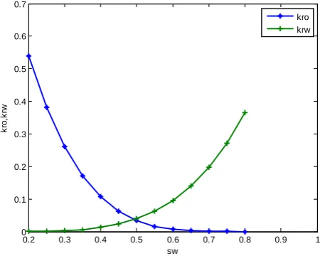
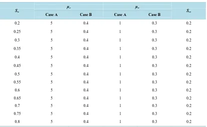
Table 6shows the values of water saturation and viscosities for Case A (hypothetical reservoir data) and Case B (Nigerian reservoir data) from which the relative permeability curves for cases A and B are plotted respec-tively (see Figure 3and Figure 4).

Figure 3. Graph of kro and krw against Sw for Case A. Effective and

corres-ponding relative permeability as functions of water saturation for Case A.

0.2 0.3 0.4 0.5 0.6 0.7 0.8 0.9 1

0 0.1 0.2 0.3 0.4 0.5 0.6 0.7

sw

k

ro

,k

rw

[image:17.595.171.428.83.293.2]

Figure 4. Graph of kro and krw against Sw for Case B. Effective and

[image:17.595.92.505.348.602.2]

corresponding relative permeability as functions of water saturation for Case B.

Table 6. Water saturations and viscosities for Cases A and B.

Sw

µo µw

Sro

Case A Case B Case A Case B

0.2 5 0.4 1 0.3 0.2

0.25 5 0.4 1 0.3 0.2

0.3 5 0.4 1 0.3 0.2

0.35 5 0.4 1 0.3 0.2

0.4 5 0.4 1 0.3 0.2

0.45 5 0.4 1 0.3 0.2

0.5 5 0.4 1 0.3 0.2

0.55 5 0.4 1 0.3 0.2

0.6 5 0.4 1 0.3 0.2

0.65 5 0.4 1 0.3 0.2

0.7 5 0.4 1 0.3 0.2

0.75 5 0.4 1 0.3 0.2

0.8 5 0.4 1 0.3 0.2

Table 7 shows the values of fractional flow and water saturation in the reservoir for Case A and Case B. These values are used to obtain fractional flow plots for both Cases A and B as shown inFigure 5.

Figure 3shows the saturation dependence of the effective permeabilities of oil and water. The plot shows both permeabilities as functions of the water saturation alone since the oil saturation is related to the water satu-ration by a simple relationship So = 1 − Sw. On the effective permeability of water (krw) curve, Sw = Swc = 0.2 on

the Swaxis. At Sw = 1, kw= 1.0. Similarly, for the effective permeability for oil curve Sw = Swc = 0.2 At Sw = 1, kro

= 0.55. The curves are used to describe the displacement of oil by water taking into consideration the manner in which the fluid saturations are distributed with respect to thickness as they simultaneously move through the re-servoir. Surfactants dissolved in minute quantities of water have significant effect on displacement of oil and in-

0.2 0.3 0.4 0.5 0.6 0.7 0.8 0.9 1

0 0.1 0.2 0.3 0.4 0.5 0.6 0.7 0.8 0.9 1

sw

k

ro

,k

rw