Munich Personal RePEc Archive
An Alternative to the BDS Test:
Integration Across the Correlation
Integral
Kocenda, Evzen
September 1996
Online at
https://mpra.ub.uni-muenchen.de/70510/
$7HVWIRULLG5HVLGXDOV
%DVHGRQ,QWHJUDWLQJ2YHUWKH&RUUHODWLRQ,QWHJUDO
(Y©HQ.R³HQGD
&(5*((,3UDJXH&]HFK5HSXEOLF
$EVWUDFW
7KLV SDSHU SUHVHQWV D QHZ PHWKRG RI WHVWLQJ IRU LLG 7KH WHVW LV VXJJHVWHG DV DQ
DOWHUQDWLYHWRWKHQRQSDUDPHWULF%'6WHVWZKLFKUHTXLUHVDSUR[LPLW\SDUDPHWHUε
DQGDQHPEHGGLQJGLPHQVLRQPWREHFKRVHQDUELWUDULO\$OLPLWHGVWDWLVWLFDOWKHRU\ H[LVWVWRGHWHUPLQHWKHULJKWFKRLFHRIWKHVHSDUDPHWHUV7KHSUHVHQWHGPHWKRGDLPV WR HOLPLQDWH VXFK LQGHFLVLYHQHVV E\ LQWHJUDWLRQ RYHU WKH FRUUHODWLRQ LQWHJUDO 7KH 0RQWH&DUORVLPXODWLRQLVXVHGWRWDEXODWHFULWLFDOYDOXHV RI WKH QHZ VWDWLVWLF ,Q D FRPSDUDWLYH DQDO\VLV WKH SUHVHQWHG WHVW LV DEOH WR ILQG QRQOLQHDU GHSHQGHQFLHV LQ FDVHVZKHUHWKH%'6WHVWGRHVQRWILQGWKHP7KHWHVWEHFRPHVPRUHFULWLFDOWRWKH TXHVWLRQZKHWKHUWKHGDWDLVWUXHZKLWHQRLVH
$EVWUDNW
9³OgQNXMHSRSLVRYgQDQRYgPHWRGDWHVWRYDQmQH]gYLVOkKR D LGHQWLFNkKR UR]GÀOHQm LLG 7HVW MH QDYU©HQ MDNR DOWHUQDWLYD N QHSDUDPHWULFNkPX WHVWX %'6 NWHU¬
Y\©DGXMH DE\ SDUDPHWU SUR[LPLW\ ε D SURVWRURYg GLPHQ]H P E\O\ ]YROHQ\
DUELWUgOQÀ.GLVSR]LFLMHSRX]HQHMHGQR]QD³QgVWDWLVWLFNgWHRULHMDNQHMOkSHY\EUDW W\WRGYDSDUDPHU\1DYU©HQgPHWRGD QDEm]m RGVWUDQÀQm WkWR QHUR]KRGQRVWL SRPRFm LQWHJUDFHSÎHV NRUHOD³Qm LQWHJUgO .ULWLFNk KRGQRW\ QRYk VWDWLVWLN\ MVRX WDEXORYgQ\ SRPRFm0RQWH&DUORVLPXODFH.RPSDUDWLYQmDQDO¬]DGRND]XMH©HQDYUKRYD¬WHVWMH VFKRSHQQDMmWQHOLQHgUQm]gYLVORVWLYSÎmSDGHFKNGHMHWHVW%'6ML©QHQDFKg]m1RY¬ WHVWVHWDNVWgYgSÎmVQÀM§mPNRWg]FH]GDMVRXGDWDVNXWH³QÀSRXK¬EmO¬§XP
.H\ZRUGVFKDRVQRQOLQHDUG\QDPLFVFRUUHODWLRQLQWHJUDO 0RQWH&DUORH[FKDQJHUDWHV$5&+
-(/&ODVVLILFDWLRQ&&)
,ZRXOGOLNHWRWKDQN''HFKHUWZKRVHKHOSZLWKWKLVSDSHUZDVVXEVWDQWLDO
1. Introduction
Applications of deterministic nonlinear dynamics and chaos theory to the analysis
of stochastic economic time series are widely used in contemporary macroeconomics and
finance. A broad pioneering volume on the complexity of the economy edited by
Anderson, Arrow and Pines (1988) includes a paper by Brock (1988) that is closely
related to the previously mentioned topic. A recent result in this trend is a non parametric
method of testing for nonlinear patterns in time series devised by Brock, Dechert and
Scheinkman (1987) and further developed in Brock, Dechert, Scheinkman and LeBaron
(1996). The method is known as the BDS test. Its null hypothesis is that data in a time
series is independently and identically distributed (iid). The test is unique in its ability to
detect nonlinearities while not being affected by linear dependencies in the data.
This paper suggests an alternative testing method that aims to eliminate some
shortcomings associated with the BDS test. Both methods are based on the theoretical
concept of the correlation integral described by Grassberger and Procaccia (1983). In
order to conduct the BDS test, certain parameters of it must be chosen arbitrarily, ex ante.
A limited statistical theory exists on how to determine these parameters. An erroneous
choice of them is thus likely to occur. The proposed alternative is constructed in a way
that, to a large extent, eliminates necessity of such an arbitrary choice. Empirical
comparison shows that the alternative test is more critical as it finds remains of
nonlinearities where the BDS test does not.
The paper is organized in the following manner. Section 2 provides a brief
theoretical background on why the alternative test is suggested. Section 3 describes
tabulate critical values of the newly designed statistic for different significance levels to
enable hypothesis testing. Section 4 presents power tests and puts forth an empirical
comparison. Several studies are replicated and the original results of the BDS test are
compared with those of the suggested alternative. Section 5 briefly concludes.
2. Theoretical Background
Chaotic systems of low complexity can generate seemingly random numbers that
may successfully mimic white noise and do not reveal their true nature. Under presumed
randomness, a nonlinear pattern can hide without being detected. Exchange rates, stock
market returns and other macroeconomic variables of generally high frequency are likely
to originate from low complexity chaos. Detection of nonlinear hidden patterns in such
time series provides important information about their behavior and improves the
forecasting ability over short time periods. However, a potent testing procedure is needed
at first.
It is widely acknowledged that the best known technique for the analysis of
chaotic systems is the correlation dimension. This is because of an easy computation and
the availability of a sampling theory. The test developed by Brock, Dechert, and
Scheinkman (1987), further referred to as the BDS test, is based on the mentioned
technique and was designed to detect hidden patterns in stochastic time series. It was
recently explicated to the fullest extent in Brock, Dechert, Scheinkman, and LeBaron
(1996) which can serve as a detailed reference. The method uses the concept of the
correlation integral, employed by Grassberger and Procaccia (1983), to distinguish
at a reasonable length, the reader should refer to the references cited in this section for
more profound theoretical background.
The BDS statistic is defined as
( )
[
( ) ( )]
( )BDSm T, ε =T C12 m T, ε −C,T ε m /σm T, ε
1 (1)
where Cm,T(ε) is a value of a correlation integral or a number of clustered pairs lying
within a particular tolerance distance ε at a spatial dimension m, and σm T, ( )ε is a standard
deviation of the statistic that varies with dimension m. The proximity parameter ε is
chosen arbitrarily and is chiefly enumerated as a ratio of the sample’s standard deviation.
The BDS test is a nonparametric test of the null hypothesis that the data is
independently and identically distributed (iid) against an unspecified alternative. The test
enables one to test for nonlinear dependence because it is not affected by linear
dependencies in the data. The employed procedure has power against both deterministic
and stochastic systems. The ability of this test to deal with stochastic time series makes it
strongly appealing for its application in modern macroeconomics and financial
economics.
The main feature of this test is its ability to detect nonlinear patterns in the data,
an obvious improvement over linearly oriented tests. Further detailed explanation and
application of the BDS test can be found in the original paper as well as in representative
studies by Brock and Dechert (1988), Hsieh (1989), Hsieh (1991), Brock, Hsieh and
LeBaron (1993), and Brock, Dechert, Scheinkman and LeBaron (1996).
By using pairs of histories that cluster together within a specific distance ε too
randomly distributed data. A “pattern” is defined as a repetitive occurrence of two
histories that lie within a certain distance ε of each other for different spatial (embedding)
dimensions m.
While the BDS statistic is easy to compute, only a limited statistical theory exists
on how to determine the optimal proximity parameter. If ε is too large, then all the points
are closer than ε, giving a constant value of correlation integral for every m. However, if ε is too small, then correlation integral captures too few points and yields inaccurate
estimates. One approach to taking ε to zero with increasing sample size is described in
Dechert (1994). Another is to chose ε that maximizes power against some particular
alternative. Brock, Dechert, Scheinkman and LeBaron (1996) showed that for any ε for
which K( )ε −C( )ε 2 >0, it is the case that the BDS statistic is asymptotically normal.1 In
principle, it means that the results are independent of the choice of ε. However, in
practice, the rate of convergence may depend on the value of ε. Thus, which value of ε
gives us the “best” test is a legitimate question to ask. Usually ε is enumerated as a
fraction of the standard deviation of the sample.
Another parameter that appears in the BDS statistic is m, representing the
embedding or spatial dimension. The choice of the parameter depends on which lag the
investigator wishes to test for dependence. DeLima (1992) developed a class of statistical
tests of iid which “integrate” over m and ε but still preserve the invariance property.
Another approach for the choice of m can be characterized as: higher the order of
underlying pattern in a time series, the larger magnitudes of m should be included in the
1
test. However, the order of pattern is likely to be unknown. The main problem is that that
as we increase m, then fewer and fewer non-overlapping m-histories will be available. It
means that for samples of moderate size only a low-dimensional chaos will be
characterized.
Heretofore, the BDS statistic has been calculated only for a few values of the
proximity parameter (tolerance distance) which appears in the statistic and must be chosen
arbitrarily prior the test is conducted. This was brought about, in part, by the Monte Carlo
studies of Hsieh and LeBaron (1988) who tested the asymptotic normally of the statistic for
only three values of the parameter. The fact that the BDS statistic is calculated for only a
few values of proximity parameter is not in the spirit of the Grassberger-Proccacia
correlation integral (on which the statistic is based) which is typically calculated over a
broad range of the proximity parameter, and in particular for a number of small values of
the parameter.
It is the aim of this paper to propose an alternative testing method that eliminates
the above mentioned shortcomings. Minimizing indecisiveness of what the proper
distance ε and spatial dimension m should be seems to represent the avenue to go.
3. An alternative test
Let
{ }
xt be a scalar time series of length T. Form m-dimensional vectors, calledm-histories, xtm =
(
x xt, t+1,...,xt m+ −1)
. Such m-dimensional vectors are used to calculatecorrelation integral at embedding dimension m which is given by
( )
(
)
(
(
)
)
Cm T I x x T T
t T
s t T
t m
s m
m m
m m
, ε = ε , ⋅ / −
= = +
−
∑ ∑
1 1
1
where Tm = − +T m 1, and I x
(
t x)
ms m
ε , is an indicator function of event
xtm xsm x x
i m t i s
− = − <
=sup0,..., −1 + +1
ε (3)
Thus the correlation integral measures fraction of pairs that lie within the tolerance
distance ε for particular spatial dimension m. Grassberger and Procaccia (1983) used
correlation integral to define the correlation dimension
( )
(
)
ν ε ε
ε
m = Cm
→
lim log / log
0 (4)
for small values of ε. If νm does not increase with m, then the data are consistent with
chaotic behavior.
The alternative test is based on the correlation integral described by equations (2,
3). However, it is configured in a manner that radically differs from the way how the
BDS statistic is constructed. In order to minimize indecisiveness on what a proper
tolerance distance should be, the method suggests the use of a number of tolerance
distances for each particular spatial dimension. The tolerance distances are chosen from
within a specific range. The alternative statistic is constructed as follows.
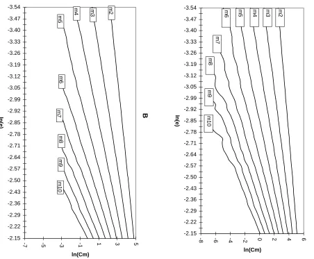
The log of the correlation integral, ln(Cm(ε)), is plotted against the log of the
proximity parameter, ln(ε), for particular spatial dimension m. Because numerous
tolerance distances ε are used, then such a plot yields a map of trajectories as illustrated
in Figure 1a. Such a representation was used in a conditional variance analysis of
exchange rates in Koûenda (1996). These trajectories decrease under different slopes that
lying within the tolerance distance results in increased variance, and the far sections of
the trajectories become highly erratic. If a larger number of matched pairs had been
included, the variance would asymptotically decrease and the erratic portion of the
trajectories would straighten. However, this can be accomplished only by providing an
infinite sample of observations. In order to preserve the sections with a constant slope,
Cm(ε) is constrained accordingly. The map of trajectories then look like one depicted in a
Figure 1b.
To summarize, an alternative test of the iid hypothesis is developed by calculating
the slope of the log of the correlation integral versus the log of the proximity parameter over
a broad range of values of the proximity parameter. The slope coefficients will be called
βm and can be calculated as
( ) ( )
(
)
(
(
( ))
(
( ))
)
( ) ( )(
)
β
ε ε ε ε
ε ε
ε
ε
m
m m
C C
=
− −
−
∑
∑
ln ln ln ln
ln ln 2
(5)
where ln(ε) is the log of proximity parameter (tolerance distance), ln(Cm(ε)) is the
correlation integral value, and m is embedding dimension.
As it is evident from their construction, the slope coefficients βm have an
interesting feature. A whole range of different tolerance distances ε is used and slope
coefficients are computed over the specified interval. Therefore, slope coefficients βm do
not depend on the arbitrary choice of the distance ε. Thus, inadequate choice of ε is
almost eliminated, and the precision of hypothesis testing is highly increased. The same
which gives enough variety to capture more complex dimensional structure without
eliminating some unexplored opportunity.
One theoretical feature of the slope coefficients βm is that under the null
hypothesis, the data is iid, and these slopes should equal the respective embedding
dimension m at which the statistic is calculated (i.e. βm = m).2 However, slope coefficient
estimates of βm are smaller than respective spatial dimension m, i.e. βm < m. This is
because of the following. From (1) and (2) it follows that
( )
(
) (
)
lim ,
T m T s t
m
E C P X X
→∞ ε = − <ε (6)
Taking natural logarithm of both sides yields
( )
(
)
(
)
lim ln , ln
T→∞ E Cm T ε = ⋅m P Xs −Xt <ε (7) Since
(
)
( )
( ) ( )P Xs Xt f y f x dydx f x dx
x x
− < =
∫
∫
≅∫
− + −∞ ∞ ε ε ε ε 2 2 ( ) ( ) (8)
is true for small ε. Hence,
(
)
( ) lim ε ε ε → − < =∫
≡ 0 2 2P X X
f x dx k s t (9) and
(
)
lim ln ln ε ε ε → − < = 0P Xs Xt
1 (10)
By Jensen’s inequality
( )
(
)
(
( ))
Eln Cm T, ε ≤lnE Cm T, ε (11)
2
It follows that for large T and small ε,
( )
(
)
(
( ))
( ) ( )Eln Cm T, ε <lnE Cm T, ε ≅mln k +mlnε (12)
As in the regression
( )
(
)
( )ln Cm T, ε = +α β εln +e (13)
the left hand variable has a negative bias from
( ) ( )
mln k +mln ε (14)
Therefore, the smaller ε is, the smaller the bias, so that the estimated coefficient satisfies
[ ]
Eβ < m (15)
This completes the explanation of the nature of the slope coefficients estimates (βm) being
smaller than respective spatial dimension (m).
How do the slope coefficients βm compare to the BDS statistic with reference to
their decipherable abilities? The BDS statistic is supposed to stay within a certain
confidence interval if the data is white noise. The intuition behind the slope coefficients
βm is similar. If the data is identically and independently distributed then the slope
coefficients βm must stay within certain confidence intervals as well. Therefore, in order
to derive the statistical properties of this test, a Monte Carlo study of the distribution of
these slopes under the null hypothesis is performed.
The confidence intervals of the slope coefficients βm were calculated using a
Monte Carlo technique with 3,000 and 2,000 replications, depending on the length of the
white noise time series. In order to obtain the “whitest” white noise observations, a
(1987) and is constructed from 17 generators described by Fishman and Moore (1982).
This method was chosen for two reasons. First, the method of a compound random
numbers generator effectively eliminates repetitiveness in the data which is caused by the
limitations of the computer hardware. Secondly, other methods, such as obtaining
hypothetically white noise residuals by estimating a generating process (i.e. AR, ARCH,
GARCH etc.) may possess some unaccounted for structural form which would bias the
critical values in a Monte Carlo simulation.
The simulations generated groups of iid samples containing 500, 1000, and 2500
observations distributed normally with a zero mean and unit variance. Each sample was
exposed to the computational procedure of correlation integral allowing for nine
embedding spatial dimensions m (2-10) and 41 tolerance distances ε ranging over the
interval 0 25 10. σ σ, . by equal increments. Then, slope coefficient estimates of βm were
calculated according to the equation (5).
To obtain the most accurate slope coefficient estimates of βm of the constant slope
portions of the trajectories, a cut-off point was set. This was done in order to eliminate the
erratic portion of the trajectories at the highest spatial dimensions m (7-9). The value of
correlation integral was constrained to be 50 by empirical examination of different plots
of trajectories resulting from a previous research.3 Such a cut-off point does not affect the
analysis for lower spatial dimensions m at all, however, considerably helps to reduce the
increasing variance as spatial dimension m grows larger and tolerance distance ε becomes
smaller. At this moment the value of correlation integral becomes so erratic that only
3’Cut-off’ value for C
notable increases in a number of replications could cure the roughness, and hence, lessen
the variance.
Finally, quantiles for slope coefficient estimates βm at different dimensional levels
were tabulated.4 Table 1 presents the quantiles to allow a hypothesis testing at levels of 1,
2, 5, and 10 percents for a time series of 500 observations. Tables 2 and 3 present the
quantiles for a time series of the length 1000 and 2500 observations, respectively. Let Lα
and Uα be lower and upper bounds of the (100 - α) percentage confidence interval of the
distribution. If
(
x<Lα) (
∨ x>Uα)
, then null hypothesis of iid can be rejected at the αpercent confidence level.
4. Power Tests and Empirical Comparison
4.1 Power Tests
The power of the method is tested against some nonlinear data resulting from
processes described below. Their choice is based on their common use, and the fact that
they do not contain any linear structure. This eliminates the problem of removing linear
structure by taking residuals of a fitted linear model.
The first model used is the nonlinear moving average (NLMA) in the following
form:
xt =5ε εt−1 t−2 +εt (16)
4The ‘slope test’ does not simultaneously test that β
The εt terms are iid normal. The second model is the ARCH model of Engle (1982) that
can be represented in the following form:
( )
xt ~N 0,ht (17)
ht ixt i
i q
= + −
=
∑
α0 α
2 1
where in this case q = 1, α0 = 1, and α1 = 0.5.
Table 4 shows the power of the test against specific models for lengths of 500,
1000, and 2500 observations. The numbers represent the frequency of rejection at the 5%
confidence level. Derivation of critical values is described in the previous section. Power
of the test against specified models is comparable with the power of the BDS statistic
shown in Hsieh and LeBaron (1988) and Brock, Dechert, Scheinkman, and LeBaron
(1996). However, due to the characteristics of the correlation integral, the power naturally
declines at the highest levels of embedding dimension.
Series that exhibit zero autocorrelation structure, as the above models do, are
rarely found in practical application. The suggested method is, therefore, meant as a
residual diagnostic for empirical analysis. The following examples of empirical
comparisons suggest the usefulness and added value of the proposed testing method.
4.2 Empirical Comparison
High frequency financial data reflect fully a stylized fact of changing variance
over time. Numerous financial time series were studied and found to contain linear as
well as non-linear dependencies. An appropriate model that would account for
nonlinear patterns in the data. Standardized (fitted) or corrected residuals from such a
model are an ideal material to be confronted with the BDS test as well as with the
suggested alternative method because if the null model is correctly specified, then those
residuals should be independent. In other words, they should not contain any other useful
forecastable structure. Thus, the test can be used not only as a test for nonlinearity but as
a correct specification test as well.
Four empirical studies were chosen to be replicated in order to yield comparisons
between the two tests. Notation throughout this section is kept for clarity as in original
studies. Results show that suggested alternative is able to detect remaining non-linear
dependencies in standardized (fitted) residuals where the BDS test does not.
4.2.1 Analysis of weekly exchange rates
Kugler and Lenz (1990) analyzed non-linear dependence of exchange rate changes
for four currencies against the US dollar. They used weekly end of period data of
Deutsche Mark (DMUS), Swiss Franc (SFUS), French Franc (FFUS), and Japanese Yen
(YNUS). The sample period is 1979-1989 and has T = 575 observations for the rate of
change of the log exchange rate xt = ∆logSt. The LM test performed on the rate of
changes clearly indicates presence of autoregressive conditional heteroskedasticity, and
the BDS test decisively rejects the null of iid. The data was corrected to account for the
ARCH process by transformation into the ARCH corrected rate of changes in a form
∆ ∆
∆
log log
$ $ log
.
S S
S t
h t
t
= +
= −
∑
α ατ
τ τ
0 1 6
2
where α-coefficients were obtained by OLS regression of ( log∆ St)2 on constant and six
lagged variables. Such ARCH corrected rate of changes were subjected to the BDS test
using spatial dimensions N = 2,3,4, and 5, and tolerance distances ε = 0.5, 0.75, 1.0, and
1.5 of the standard deviation of the sample. Kugler and Lenz (1990) found that the
described correction successfully removed nonlinearity from the Swiss Franc and
Deutsche Mark. However, the BDS test did not allow rejection of the null hypothesis for
the French Franc (specifically at levels of N = 4 and 5) and Japanese Yen (specifically at
levels of N = 3,4, and 5).
I have replicated the original study with the same results and applied the corrected
rates to the alternative test. The results are presented in Table 5. As in the original study,
the null hypothesis is rejected for the French Franc and Japanese Yen. Contrary to the
original analysis, the alternative test finds remaining non-linear dependency in the
residuals of the Deutsche Mark. Swiss Franc is the only currency where the null of iid
cannot be rejected. The alternative test confirmed presence of non-linearity in the
corrected residuals of the French Franc and Japanese Yen, and detected remaining
dependency in presumably independent Deutsche Mark.
4.2.2 Analysis of daily exchange rates
Brock, Hsieh, and LeBaron (1993), p. 130, analyzed daily closing bid prices of the
five major currencies in U.S. Dollars: Swiss Franc (SF), Canadian Dollar (CD), Deutsche
2, 1974 to December 30, 1983.5 The length of the time series is 2,510 observations. The
analysis was based on Hsieh (1989).
As in the original study, the rates of change are calculated by taking the first
logarithmic differences between successive trading days. The data were prefiltered by an
autoregressive process with daily dummies to remove linear dependency. In order to
capture variance-nonlinearity a GARCH model of exchange rates was estimated. The
specification of the model resulted into the following mean equation:
rt i t ir MDM t TDT t WDW t RDR t HDH ut i
j
= + − + + + + + +
=
∑
β0 β β β β β β
1
, , , , (19)
where, ut|Ωt−1 ~ D( ,0 ht), and variance equation
ht =φ0+ψu2t−1+φht−1+φMDM t, +φTDT t, +φWDW t, +φRDR t, +φHDH (20)
where rt is a rate of change of the nominal exchange rate at time t, and DM,t, DT,t, DW,t,
and DR,t, are dummy variables for Monday, Tuesday, Wednesday, and Thursday, and DH
is the number of holidays between two successive trading days excluding week-ends.
Daily dummies were included to capture the daily effects of fluctuations that are known
to materialize in correlation at financial markets and thus might affect the analysis. The
order of an autoregressive process is determined to be j = 6, 5, 6, and 0 respectively for
SF, CD, DM, and BP.
The BDS test was performed on the raw data as well as on the prefiltered data.
The results in both cases do not differ. The data are not white noise. After estimation, the
overall fit of the model is accessed by performing diagnostic tests on standardized
residuals zt =ut /ht12 where u
t is the residual of the mean equation (19), and ht is the
5
estimated conditional variance from equation (20). The BDS test finds no evidence of
nonlinearity in standardized residuals of SF, some nonlinearity (at dimensions 8, 9, and
10) for the DM, and strong nonlinearity for CD and BP.
Replicated findings are in accordance with the above stated findings of Brock,
Hsieh, and LeBaron (1993), pp. 140 and 155.6 Then, the standardized residuals are
subjected to the alternative test. The slope coefficients derived from the test on
standardized residuals are presented in the Table 6. DM and BP show presence of
nonlinearity at the 1% significance level no matter what embedding dimension is
considered. CD and SF show some presence of nonlinearity at various significance levels
depending on spatial dimension m. The alternative test confirmed the presence of
nonlinearity in DM, CD, and BP and, contrary to the original study, detected remaining
nonlinearity in supposedly independent residuals of SF.
4.2.3 Analysis of weekly exchange rates
Kugler and Lenz (1993) analyzed non-linear dependence of exchange rate changes
for ten currencies against the US dollar. They used weekly end of period data of
Australian dollar (ADUS), Canadian dollar (CDUS), Belgian Franc (BFUS), French
Franc (FFUS), Deutsche Mark (DMUS), Dutch Guilder (HFUS), Italian Lira (LTUS),
Spanish Peseta (PTUS), Swiss Franc (SFUS), and Japanese Yen (YNUS). The sample
period is 1979-1989 and has T = 575 observations for the rate of change of the log
exchange rate xt = ∆logSt. The LM test performed on the rate of changes clearly
indicates the presence of autoregressive conditional heteroskedasticity, and the BDS test
decisively rejects the null of iid. In order to check whether the detected dependence can
be solely attributed to an ARCH process, they estimated the following GARCH-M model
∆logSt = + +∆logSt + ht + t
= −
∑
β βτ β η
τ τ
0 1 3
4 (21)
ht =α0 +α η1 2t−1+α2ht−1 ηt =εt ht
In equation (21) linear dependencies of the AR type are allowed for, as the estimated pure
GARCH-M model showed signs of residual autocorrelation for some currencies. For all
currencies the GARCH coefficients α$1 and α$2 are highly significant from zero. Thus
ARCH effects are important for all currencies. Finally, the fitted residuals ε$t =ηt / ht
were subjected to the BDS test (tolerance distance of one standard deviation and
embedding dimensions N = 2,3,4, and 5 were used). Results revealed that there was no
indication of dependence in the fitted residuals of any currency.
I have replicated the study with the same results. Then, the fitted residuals ε$t were subjected to the alternative test. The results, that are presented in Table 7, confirmed the
original findings for five out of ten currencies being independent (CDUS, FBUS, FFUS,
HFUS, and SFUS). However, contrary to the original analysis, the alternative method
was able to detect remaining non-linear dependencies in fitted residuals for the rest of
supposedly independent currencies (ADUS, DMUS, LTUS, PTUS, and YNUS).
4.2.4 Analysis of daily stock market index
Olmeda and Perez (1995) explored the existence of non-linear dynamics and
chaos in the Spanish stock market. Their database is composed of 1256 observations
(from January 2, 1989 to January 31, 1994) of the General Index of Madrid’s Stock
Market, not corrected for dividends or splits. Using the BDS test they found that the
returns series shows significant linear and non-linear dependence. They estimated a
GARCH (1,1) model for AR(1) residuals in a form
xt = σtut, σt α α xt βσt
2
0 1 1 2
1 2
= + − + − , ut ~N
( )
0 1 (22),and formed the standardized residuals st =et /σt of this model. They found that the BDS
statistic values were still significant at 5% level, showing that the GARCH (1,1) model
could not account for all the nonlinearity.
The estimation was replicated with the equal results and then the standardized
residuals were subjected to the alternative test. The results are presented in Table 8. It is
evident that the null hypothesis of iid can be decisively rejected at 1% level. The test thus
even strongly confirmed original findings.
5. Conclusion
This paper has presented a new method of testing for iid. The method originates in
a chaos theory and is based on the concept of the correlation integral. The test is
suggested as an alternative to a widely used nonparametric BDS test. The BDS test
requires two parameters, proximity parameter ε and embedding dimension m, to be
chosen arbitrarily ex ante. Only a limited statistical theory exists to determine the right
choice of these parameters for particular data set. Presented new method eliminates, to a
correlation integral. An alternative statistic is developed by calculating the slope of the log
of the correlation integral versus the log of the proximity parameter over a broad range of
values of the proximity parameter for different embedding dimensions. The Monte Carlo
simulation is used to tabulate critical values of the slope coefficients βm at different
significance levels.
The power of the new method is tested against some nonlinear artificial data. A
comparative analysis of four empirical studies is executed in order to evaluate its
performance. The presented test is applied on standardized or corrected residuals from
different models and is able to find nonlinear dependencies in cases where the BDS test
does not find them. Thus, the alternative test becomes more critical to the question
whether the data is true white noise or whether some nonlinear pattern hides undetected
within a time series.
The importance of having a good test for detecting nonlinearity in a time series
and especially in the residuals from the null model is ever more important with the
increasing number of sophisticated quantitative methods being implemented into finance
and macroeconomics. The proposed methodology with increased sensitivity is believed to
F igure 1 Traj ect ori es of t h e pl ot te d l n (C m ( ε
)) against ln(
ε ) at vari ous s p at ia l di mens ions m (A) Uncons trai
ned and (B
) C ons trai ned C as es A
-8 -6 -4 -2 0 2 4 6
-3.54 -3.47 -3.40 -3.33 -3.26 -3.19 -3.12 -3.05 -2.99 -2.92 -2.85 -2.78 -2.71 -2.64 -2.57 -2.50 -2.43 -2.36 -2.29 -2.22 -2.15 ln (e ) ln(Cm) m2 m3 m4 m5 m6 m7 m8 m9 m1 0 B
-7 -5 -3 -1 1 3 5
References
Anderson, P. W., Arrow, K. J., and Pines, D., editors, 1988, The Economy as an Evolving Complex System, Santa Fe Institute Studies in the Sciences of Complexity, v. 5
(Addison-Wesley Publishing Company)
Bollerslev, T., 1986, Generalized Autoregressive Conditional Heteroskedasticity, Journal
of Econometrics, 31, 307-327.
Brock, W., 1988, Nonlinearity and Complex Dynamics in Economics and Finance in Anderson, P. W., Arrow, K. J., and Pines, D., editors, 1988, The Economy as an Evolving Complex System, Santa Fe Institute Studies in the Sciences of Complexity, v. 5 (Addison-Wesley Publishing Company)
Brock, W., and Dechert, W., 1988, A General Class of Specification Tests: The Scalar Case, in Business and Economics Statistics Section of the Proceeding of the American
Statistical Society, pp. 70-79.
Brock, W., Dechert, W., and Scheinkman, J., 1987, A Test for Independence Based on the Correlation Dimension, University of Wisconsin at Madison, Department of Economics Working Paper.
Brock, W., Dechert, W., Scheinkman, J., and LeBaron, B., 1996, A Test for
Independence Based on the Correlation Dimension, forthcoming in Econometric
Reviews
Brock, W. A., Hsieh, D. A., and LeBaron, B., 1993, Nonlinear Dynamics, Chaos, and Instability: Statistical Theory and Economic Evidence, The MIT Press, Cambridge, Massachusetts
Collings, B. J., 1987, Compound Random Number Generators, Journal of the American
Statistical Association, 82, Theory and Methods, 525-527
Dechert, W. D., 1994, The Correlation Integral and the Independence of Gaussian and Related Processes, SSRI Working Paper 9412, University of Wisconsin-Madison
DeLima, P., 1992, A Test for IID Based upon the BDS Statistic, Department of Economics, Johns Hopkins University
Engle, R. F., 1982, Autoregressive Conditional Heteroskedasticity with Estimates of the Variance of United Kingdom Inflation, Econometrica, 50, 987-1007.
Fishman, G. S., and Moore, L. R., 1982, A Statistical Evaluation of Multiplicative Congruential Random Number Generators with Modulus 231-1, Journal of the
Grassberger, P., and Procaccia, I., 1983, Measuring the Strangeness of Strange Attractors, Physica 9D, 189-208.
Hsieh, D. A., 1989, Testing for Nonlinear Dependence in Daily Foreign Exchange Rates,
Journal of Business 62, 339-368.
Hsieh, D. A., 1991, Chaos and Nonlinear Dynamics: Application to Financial Markets,
Journal of Finance 46, 1839-1877.
Hsieh, D. A., and LeBaron, B., 1988, Finite Sample Properties of the BDS Statistic, University of Chicago and University of Wisconsin-Madison, in Brock, W. A., Hsieh, D. A., and LeBaron, B., Nonlinear Dynamics, Chaos, and Instability: Statistical Theory and Economic Evidence, The MIT Press, Cambridge, Massachusetts, 1993
Koûenda, E., 1997, Volatility of a Seemingly Fixed Exchange Rate, forthcoming in
Eastern European Economics
Kugler, P., and Lenz, C., 1990, Sind Wechselkursfluktuationen zufullig oder chaotisch? (Are Exchange Rate Fluctuations Random or Chaotic?), Schweizerische Zeitschrift fhr
Volkswirtschaft und Statistik, 126(2), 113-128
Kugler, P., and Lenz, C., 1993, Chaos, ARCH, and the Foreign Exchange Market: Empirical Results from Weekly Data, Rivista Internazionale di Scienze Economiche e
Commerciali, 40(2), 127-140